Unit 8 Supply and demand: Price-taking and competitive markets
Themes and capstone units
How markets operate when all buyers and sellers are price-takers
- Competition can constrain buyers and sellers to be price-takers.
- The interaction of supply and demand determines a market equilibrium in which both buyers and sellers are price-takers, called a competitive equilibrium.
- Prices and quantities in competitive equilibrium change in response to supply and demand shocks.
- Price-taking behaviour ensures that all gains from trade in the market are exhausted at a competitive equilibrium.
- The model of perfect competition describes idealized conditions under which all buyers and sellers are price-takers.
- Real-world markets are typically not perfectly competitive, but some policy problems can be analysed using this demand and supply model.
- There are important similarities and differences between price-taking and price-setting firms.
Students of American history learn that the defeat of the southern Confederate states in the American Civil War ended slavery in the production of cotton and other crops in that region. There is also an economics lesson in this story.
At the war’s outbreak on 12 April 1861, President Abraham Lincoln ordered the US Navy to blockade the ports of the Confederate states. These states had declared themselves independent of the US to preserve the institution of slavery.
As a result of the naval blockade, the export of US-grown raw cotton to the textile mills of Lancashire in England came to a virtual halt, eliminating three-quarters of the supply of this critical raw material. Sailing at night, a few blockade-running ships evaded Lincoln’s patrols, but 1,500 were destroyed or captured.
- excess demand
- A situation in which the quantity of a good demanded is greater than the quantity supplied at the current price. See also: excess supply.
We will see in this unit that the market price of a good, such as cotton, is determined by the interaction of supply and demand. In the case of raw cotton, the tiny quantities reaching England through the blockade were a dramatic reduction in supply. There was large excess demand—that is to say, at the prevailing price, the quantity of raw cotton demanded exceeded the available supply. As a result, some sellers realized they could profit by raising the price. Eventually, cotton was sold at prices six times higher than before the war, keeping the lucky blockade-runners in business. Consumption of cotton fell to half the prewar level, throwing hundreds of thousands of people who worked in cotton mills out of work.
Mill owners responded. For them, the price rise was an increase in their costs. Some firms failed and left the industry due to the reduction in their profits. Mill owners looked to India to find an alternative to US cotton, greatly increasing the demand for cotton there. The excess demand in the markets for Indian cotton gave some sellers an opportunity to profit by raising prices, resulting in increases in the prices of Indian cotton, which quickly rose almost to match the price of US cotton.
Responding to the higher income now obtainable from growing cotton, Indian farmers abandoned other crops and grew cotton instead. The same occurred wherever cotton could be grown, including Brazil. In Egypt, farmers who rushed to expand the production of cotton in response to the higher prices began employing slaves, captured (like the American slaves that Lincoln was fighting to free) in sub-Saharan Africa.
There was a problem. The only source of cotton that could come close to making up the shortfall from the US was in India. But Indian cotton differed from American cotton, and required an entirely different kind of processing. Within months of the shift to Indian cotton, new machinery was developed to process it.
As the demand for this new equipment soared, firms like Dobson and Barlow, who made textile machinery, saw profits take-off. We know about this firm, because detailed sales records have survived. It responded by increasing production of these new machines and other equipment. No mill could afford to be left behind in the rush to retool, because if it didn’t, it could not use the new raw materials. The result was, in the words of Douglas Farnie, a historian who specialized in the history of cotton production, ‘such an extensive investment of capital that it amounted almost to the creation of a new industry.’
The lesson for economists: Lincoln ordered the blockade, but in what followed, the farmers and sellers who increased the price of cotton were not responding to orders. Neither were the mill owners who cut back the output of textiles and laid off the mill workers, nor were the mill owners desperately searching for new sources of raw material. By ordering new machinery, the mill owners set off a boom in investment and new jobs.
All of these decisions took place over a matter of months, by millions of people, most of whom were total strangers to one another, each seeking to make the best of a totally new economic situation. American cotton was now scarcer, and people responded, from the cotton fields of Maharashtra in India to the Nile delta, to Brazil, and the Lancashire mills.
To understand how the change in the price of cotton transformed the world cotton and textile production system, think about the prices determined by markets as messages. The increase in the price of US cotton shouted: ‘find other sources, and find new technologies appropriate for their use.’ Similarly, when the price of petrol rises, the message to the car driver is: ‘take the train’, which is passed on to the railway operator: ‘there are profits to be made by running more train services’. When the price of electricity goes up, the firm or the family is being told: ‘think about installing photovoltaic cells on the roof.’
In many cases—like the chain of events that began at Lincoln’s desk on 12 April 1861—the messages make sense not only for individual firms and families but also for society: if something has become more expensive then it is likely that more people are demanding it, or the cost of producing it has risen, or both. By finding an alternative, the individual is saving money and conserving society’s resources. This is because, in some conditions, prices provide an accurate measure of the scarcity of a good or service.1
In planned economies, which operated in the Soviet Union and other central and eastern European countries before the 1990s (discussed in Unit 1), messages about how things would be produced are sent deliberately by government experts. They decide what will be produced and at what price it will be sold. The same is true, as we saw in Unit 6, inside large firms like General Motors, where managers (and not prices) determine who does what.
The amazing thing about prices determined by markets is that individuals do not send the messages, but rather the anonymous interaction of sometimes millions of people. And when conditions change—a cheaper way of producing bread, for example—nobody has to change the message (‘put bread instead of potatoes on the table tonight’). A price change results from a change in firms’ costs. The reduced price of bread says it all.
8.1 Buying and selling: Demand and supply
- willingness to pay (WTP)
- An indicator of how much a person values a good, measured by the maximum amount he or she would pay to acquire a unit of the good. See also: willingness to accept.
In Unit 7 we considered the case of a good produced and sold by just one firm. There was one seller with many buyers in the market for that product. In this unit, we look at markets where many buyers and sellers interact, and show how the competitive market price is determined by both the preferences of consumers and the costs of suppliers. When there are many firms producing the same product, each firm’s decisions are affected by the behaviour of competing firms, as well as consumers.
For a simple model of a market with many buyers and sellers, think about the potential for trade in second-hand copies of a recommended textbook for a university economics course. Demand for the book comes from students who are about to begin the course, and they will differ in their willingness to pay (WTP). No one will pay more than the price of a new copy in the campus bookshop. Below that, students’ WTP may depend on how hard they work, how important they think the book is, and on their available resources for buying books.
Often when you buy something you don’t need to think about your exact willingness to pay. You just decide whether to pay the asking price. But WTP is a useful concept for buyers in online auctions, such as eBay.
If you want to bid for an item, one way to do it is to set a maximum bid equal to your WTP, which will be kept secret from other bidders: this article explains how to do it on eBay. eBay will place bids automatically on your behalf until you are the highest bidder, or until your maximum is reached. You will win the auction if, and only if, the highest bid is less than or equal to your WTP.
- willingness to accept (WTA)
- The reservation price of a potential seller, who will be willing to sell a unit only for a price at least this high. See also: willingness to pay.
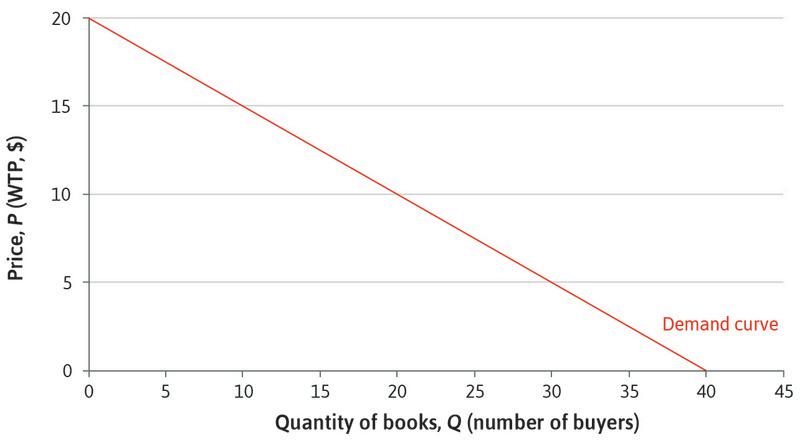
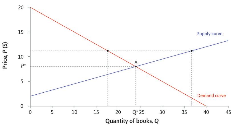
Figure 8.1 shows the demand curve. As in Unit 7, we line up all the consumers in order of willingness to pay, highest first. The first student is willing to pay $20, the 20th $10, and so on. For any price, P, the graph tells you how many students would be willing to buy: it is the number whose WTP is at or above P.
The demand curve represents the WTP of buyers; similarly, supply depends on the sellers’ willingness to accept (WTA) money in return for books.
- reservation price
- The lowest price at which someone is willing to sell a good (keeping the good is the potential seller’s reservation option). See also: reservation option.
The supply of second-hand books comes from students who have previously completed the course, who will differ in the amount they are willing to accept—that is, their reservation price. Recall from Unit 5 that Angela was willing to enter into a contract with Bruno only if it gave her at least as much utility as her reservation option (no work and survival rations); here the reservation price of a potential seller represents the value to her of keeping the book, and she will only be willing to sell for a price at least that high. Poorer students (who are keen to sell so that they can afford other books) and those no longer studying economics may have lower reservation prices. Again, online auctions like eBay allow sellers to specify their WTA.
If you sell an item on eBay you can set a reserve price, which will not be disclosed to the bidders. This article explains eBay reserve prices. You are telling eBay that the item should not be sold unless there is a bid at (or above) that price. So the reserve price should correspond to your WTA. If no one bids your WTA, the item will not be sold.
- supply curve
- The curve that shows the number of units of output that would be produced at any given price. For a market, it shows the total quantity that all firms together would produce at any given price.
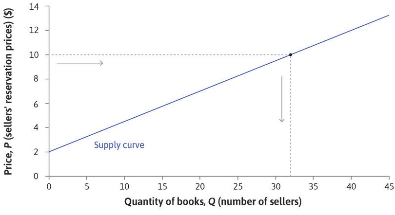
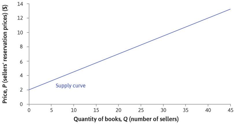
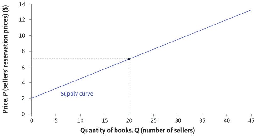
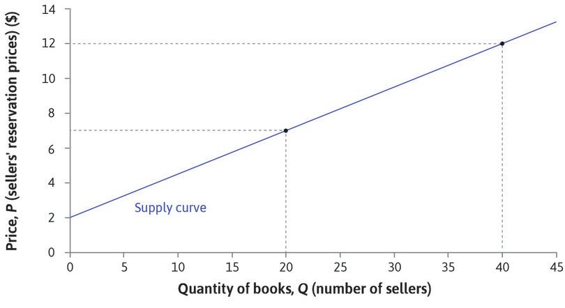
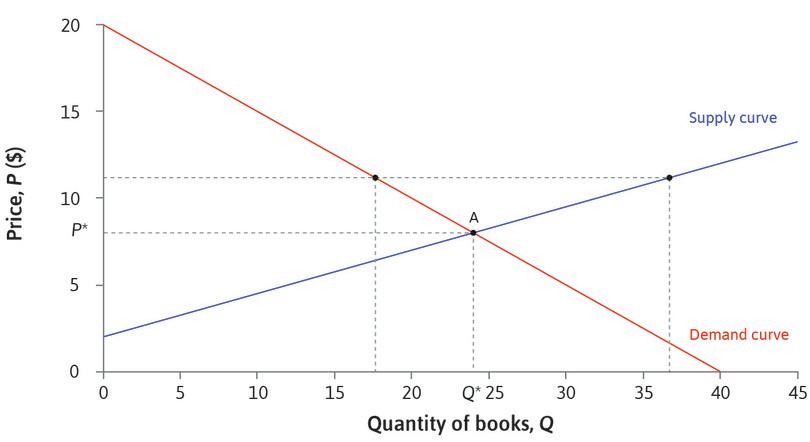
We can draw a supply curve by lining up the sellers in order of their reservation prices (their WTAs): see Figure 8.2. We put the sellers who are most willing to sell—those who have the lowest reservation prices—first, so the graph of reservation prices slopes upward.
For any price, the supply curve shows the number of students willing to sell at that price—that is, the number of books that will be supplied to the market. Notice that we have drawn the supply and demand curves as straight lines for simplicity. In practice they are more likely to be curves, with the exact shape depending on how valuations of the book vary among the students.
Question 8.1 Choose the correct answer(s)
As a student representative, one of your roles is to organize a second-hand textbook market between the current and former first-year students. After a survey, you estimate the demand and supply curves. For example, you estimate that pricing the book at $7 would lead to a supply of 20 books and a demand of 26 books. Which of the following statements is correct?
- The rumour would make the former first-year students less willing to sell. Their WTAs would rise, shifting the supply curve upwards. Equivalently, the number of students willing to supply their book at each price would be lower.
- From the supply curve, we can see that supply would double to 40 if the price were increased to $12.
- The rumour would shift the demand curve downwards.
- The maximum demand attainable is 40 at zero price.
Exercise 8.1 Selling strategies and reservation prices
Consider three possible methods to sell a car that you own:
- Advertise it in the local newspaper.
- Take it to a car auction.
- Offer it to a second-hand car dealer.
- Would your reservation price be the same in each case? Why?
- If you used the first method, would you advertise it at your reservation price?
- Which method do you think would result in the highest sale price?
- Which method would you choose?
8.2 The market and the equilibrium price
What would you expect to happen in the market for this textbook? That will depend on the market institutions that bring buyers and sellers together. If students have to rely on word-of-mouth, then when a buyer finds a seller they can try to negotiate a deal that suits both of them. But each buyer would like to be able to find a seller with a low reservation price, and each seller would like to find a buyer with a high willingness to pay. Before concluding a deal with one trading partner, both parties would like to know about other trading opportunities.
Traditional market institutions often brought many buyers and sellers together in one place. Many of the world’s great cities grew up around marketplaces and bazaars along ancient trading routes such as the Silk Road between China and the Mediterranean. In the Grand Bazaar of Istanbul, one of the largest and oldest covered markets in the world, shops selling carpets, gold, leather, and textiles cluster together in different areas. In medieval towns and cities it was common for makers and sellers of a specific type of good to set up shops close to each other, so customers knew where to find them. The city of London is now a financial centre, but evidence of trades once carried out there can be found in surviving street names: Pudding Lane, Bread Street, Milk Street, Threadneedle Street, Ropemaker Street, Poultry Street, and Silk Street.
With modern communications, sellers can advertise their goods and buyers can more easily find out what is available, and where to buy it. But in some cases it is still convenient for many buyers and sellers to meet each other. Large cities have markets for meat, fish, vegetables or flowers, where buyers can inspect and compare the quality of the produce. In the past, markets for second-hand goods often involved specialist dealers, but nowadays sellers can contact buyers directly through online marketplaces such as eBay. Websites now help students sell textbooks to others in their university.
At the end of the nineteenth century, the economist Alfred Marshall introduced his model of supply and demand using a similar example to our case of second-hand books. Most English towns had a corn exchange (also known as a grain exchange)—a building where farmers met with merchants to sell their grain. Marshall described how the supply curve of grain would be determined by the prices that farmers would be willing to accept, and the demand curve by the willingness to pay of merchants. Then he argued that, although the price ‘may be tossed hither and thither like a shuttlecock’ in the ‘higgling and bargaining’ of the market, it would never be very far from the particular price at which the quantity demanded by merchants was equal to the quantity the farmers would supply.
- excess supply
- A situation in which the quantity of a good supplied is greater than the quantity demanded at the current price. See also: excess demand.
- Nash equilibrium
- A set of strategies, one for each player in the game, such that each player’s strategy is a best response to the strategies chosen by everyone else.
- equilibrium (of a market)
- A state of a market in which there is no tendency for the quantities bought and sold, or the market price, to change, unless there is some change in the underlying costs, preferences, or other determinants of the behaviour of market actors.
Marshall called the price that equated supply and demand the equilibrium price. If the price was above the equilibrium, farmers would want to sell large quantities of grain. But few merchants would want to buy—there would be excess supply. Then, even the merchants who were willing to pay that much would realize that farmers would soon have to lower their prices and would wait until they did. Similarly, if the price was below the equilibrium, sellers would prefer to wait rather than sell at that price. If, at the going price, the amount supplied did not equal the amount demanded, Marshall reasoned that some sellers or buyers could benefit by charging some other price (in modern terminology, we would say that the going price was not a Nash equilibrium). So the price would tend to settle at an equilibrium level, where demand and supply were equated.
Marshall’s argument was based on the assumption that all the grain was of the same quality. His supply and demand model can be applied to markets in which all sellers are selling identical goods, so buyers are equally willing to buy from any seller. If the farmers all had grain of different qualities, they would be more like the sellers of differentiated products in Unit 7.
Great economists Alfred Marshall
- marginal cost
- The effect on total cost of producing one additional unit of output. It corresponds to the slope of the total cost function at each point.
- marginal utility
- The additional utility resulting from a one-unit increase of a given variable.
Alfred Marshall (1842–1924) was a founder—with Léon Walras—of what is termed the neoclassical school of economics. His Principles of Economics, first published in 1890, was the standard introductory textbook for English speaking students for 50 years. An excellent mathematician, Marshall provided new foundations for the analysis of supply and demand by using calculus to formulate the workings of markets and firms, and express key concepts such as marginal costs and marginal utility. The concepts of consumer and producer surplus are also due to Marshall. His conception of economics as an attempt to ‘understand the influences exerted on the quality and tone of a man’s life by the manner in which he earns his livelihood …’ is close to our own definition of the field.2
Sadly, much of the wisdom in Marshall’s text has rarely been taught by his followers. Marshall paid attention to facts. His observation that large firms could produce at lower unit costs than small firms was integral to his thinking, but it never found a place in the neoclassical school. This may be because if the average cost curve is downward-sloping even when firms are very large, there will be a kind of winner-takes-all competition in which a few large firms emerge as winners with the power to set prices, rather than taking the going price as a given. We return to this problem in Unit 12 and Unit 21.
Marshall would also have been distressed that homo economicus (whose existence we questioned in Unit 4) became the main actor in textbooks written by the followers of the neoclassical school. He insisted that:
Ethical forces are among those of which the economist has to take account. Attempts have indeed been made to construct an abstract science with regard to the actions of an economic man who is under no ethical influences and who pursues pecuniary gain … selfishly. But they have not been successful. (Principles of Economics, 1890)
While advancing the use of mathematics in economics, he also cautioned against its misuse. In a letter to A. L. Bowley, a fellow mathematically inclined economist, he explained his own ‘rules’ as follows:
- Use mathematics as a shorthand language, rather than as an engine of inquiry
- Keep to them [that is, stick to the maths] till you have done
- Translate into English
- Then illustrate by examples that are important in real life
- Burn the mathematics
- If you can’t succeed in 4, burn 3: ‘This I do often.’
Marshall was Professor of Political Economy at the University of Cambridge between 1885 and 1908. In 1896 he circulated a pamphlet to the University Senate objecting to a proposal to allow women to be granted degrees. Marshall prevailed and women would wait until 1948 before being granted academic standing at Cambridge on a par with men.
But his work was motivated by a desire to improve the material conditions of working people:
Now at last we are setting ourselves seriously to inquire whether it is necessary that there should be any so called lower classes at all: that is whether there need be large numbers of people doomed from their birth to hard work in order to provide for others the requisites of a refined and cultured life, while they themselves are prevented by their poverty and toil from having any share or part in that life. … The answer depends in a great measure upon facts and inferences, which are within the province of economics; and this is it which gives to economic studies their chief and their highest interest. (Principles of Economics, 1890)
Would Marshall now be satisfied with the contribution that modern economics has made to creating a more just economy?
To apply the supply and demand model to the textbook market, we assume that all the books are identical (although in practice some may be in better condition than others) and that a potential seller can advertise a book for sale by announcing its price on a local website. As at the Corn Exchange, we would expect that most trades would occur at similar prices. Buyers and sellers can easily observe all the advertised prices, so if some books were advertised at $10 and others at $5, buyers would be queuing to pay $5, and these sellers would quickly realize that they could charge more, while no one would want to pay $10 so these sellers would have to lower their price.
- market-clearing price
- At this price there is no excess supply or excess demand. See also: equilibrium.
- equilibrium
- A model outcome that is self-perpetuating. In this case, something of interest does not change unless an outside or external force is introduced that alters the model’s description of the situation.
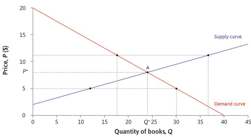
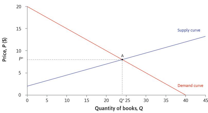
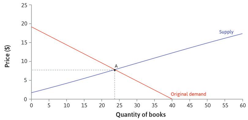
We can find the equilibrium price by drawing the supply and demand curves on one diagram, as in Figure 8.3. At a price P* = $8, the supply of books is equal to demand: 24 buyers are willing to pay $8, and 24 sellers are willing to sell. The equilibrium quantity is Q* = 24.
The market-clearing price is $8—that is, supply is equal to demand at this price, so all buyers who want to buy and all sellers who want to sell can do so. The market is in equilibrium. In everyday language, something is in equilibrium if the forces acting on it are in balance, so that it remains still. Remember Fisher’s hydraulic model of price determination from Unit 2: changes in the economy caused water to flow through the apparatus until it reached an equilibrium, with no further tendency for prices to change. We say that a market is in equilibrium if the actions of buyers and sellers have no tendency to change the price or the quantities bought and sold, unless there is a change in market conditions such as the numbers of potential buyers and sellers, and how much they value the good. At the equilibrium price for textbooks, all those who wish to buy or sell are able to do so, so there is no tendency for change.
Not all online markets for books are in competitive equilibrium. In one case when the conditions for equilibrium were not met, automatic price-setting algorithms raised the price of a book to $23 million! Michael Eisen, a biologist, noticed a classic but out-of-print text, The Making of a Fly, was listed for sale on Amazon by two reputable sellers, with prices starting at $1,730,045.91 (+$3.99 shipping). He watched over the next week as the prices rose rapidly, eventually peaking at $23,698,655.93, before dropping to $106.23. Eisen explains why in his blog.3
Price-taking
Will the market always be in equilibrium? As we have seen, Marshall argued that prices would not deviate far from the equilibrium level, because people would want to change their prices if there were excess supply or demand. In this unit, we study competitive market equilibria. In Unit 11 we will look at when and how prices change when the market is not in equilibrium.
- price-taker
- Characteristic of producers and consumers who cannot benefit by offering or asking any price other than the market price in the equilibrium of a competitive market. They have no power to influence the market price.
In the market equilibrium that we have described for the textbook, individual students have to accept the prevailing price in the market, determined by the supply and demand curves. No one would trade with a student asking a higher price or offering a lower one, because anyone could find an alternative seller or buyer with a better price. The participants in this market are price-takers, because there is sufficient competition from other buyers and sellers so the best they can do is to trade at the same price. Any buyer or seller is of course free to choose a different price, but they cannot benefit by doing so.
We have seen examples where market participants do not behave as price-takers: the producer of a differentiated product can set its own price because it has no close competitors. Notice, however, that although the sellers of differentiated products are price-setters, the buyers in Unit 7 were price-takers. Since there are so many consumers wanting to buy breakfast cereals, an individual consumer has no power to negotiate a more advantageous deal, but simply has to accept the price that all other consumers are paying.
In this unit, we study market equilibria where both buyers and sellers are price-takers. We expect to see price-taking on both sides of the market where there are many sellers selling the identical goods, and many buyers wishing to purchase them. Sellers are forced to be price-takers by the presence of other sellers, as well as buyers who always choose the seller with the lowest price. If a seller tried to set a higher price, buyers would simply go elsewhere.
- competitive equilibrium
- A market outcome in which all buyers and sellers are price-takers, and at the prevailing market price, the quantity supplied is equal to the quantity demanded.
Similarly buyers are price-takers when there are plenty of other buyers, and sellers willing to sell to whoever will pay the highest price. On both sides of the market, competition eliminates bargaining power. We will describe the equilibrium in such a market as a competitive equilibrium.
A competitive market equilibrium is a Nash equilibrium, because given what all other actors are doing (trading at the equilibrium price), no actor can do better than to continue what he or she is doing (also trading at the equilibrium price).
Exercise 8.2 Price-takers
Think about some of the goods you buy: perhaps different kinds of food, clothes, transport tickets, or electronic goods.
- Are there many sellers of these goods?
- Do you try to find the lowest price in each case?
- If not, why not?
- For which goods would price be your main criterion?
- Use your answers to help you decide whether the sellers of these goods are price-takers. Are there goods for which you, as a buyer, are not a price-taker?
Question 8.2 Choose the correct answer(s)
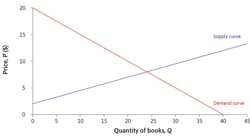
The diagram shows the demand and the supply curves for a textbook. The curves intersect at (Q, P) = (24, 8). Which of the following is correct?
- At $10 the price is above the equilibrium price of $8, and there is an excess supply of books.
- At $8, all buyers with a WTP at $8 or above can be matched with all sellers with a WTA of $8 or less. If one of these sellers raised their price to $9, the buyer could find another seller willing to accept less.
- At $8, the quantity demanded is equal to the quantity supplied—that is, the market clears.
- The maximum level of demand is 40, but 16 of these will be unfulfilled as their willingness-to-pay is below the market clearing price of $8.
8.3 Price-taking firms
In the second-hand textbook example, both buyers and sellers are individual consumers. Now we look at markets where the sellers are firms. We know from Unit 7 how firms choose their price and quantity when producing differentiated goods, and we saw that if other firms made similar products, their choice of price would be restricted (the demand curve for their own product would be almost flat) because raising the price would cause consumers to switch to other similar brands.
If there are many firms producing identical products, and consumers can easily switch from one firm to another, then firms will be price-takers in equilibrium. They will be unable to benefit from attempting to trade at a price different from the prevailing price.
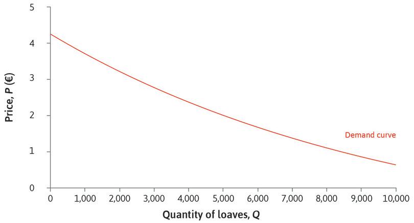
To see how price-taking firms behave, consider a city where many small bakeries produce bread and sell it direct to consumers. Figure 8.4 shows what the market demand curve (the total daily demand for bread of all consumers in the city) might look like. It is downward-sloping as usual because at higher prices, fewer consumers will be willing to buy.
Suppose that you are the owner of one small bakery. You have to decide what price to charge and how many loaves to produce each morning. Suppose that neighbouring bakeries are selling loaves identical to yours at €2.35. This is the prevailing market price, and you will not be able to sell loaves at a higher price than other bakeries, because no one would buy—you are a price-taker.
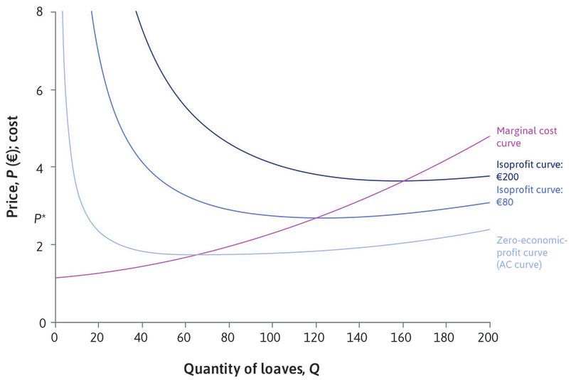
Your marginal costs increase with your output of bread. When the quantity is small, the marginal cost is low, close to €1: having installed mixers, ovens and other equipment, and employed a baker, the additional cost to produce a loaf of bread is relatively small, but the average cost of a loaf is high. As the number of loaves per day increases, the average cost falls, but marginal costs begin to rise gradually because you have to employ extra staff and use equipment more intensively. At higher quantities the marginal cost is above the average cost; then average costs rise again.
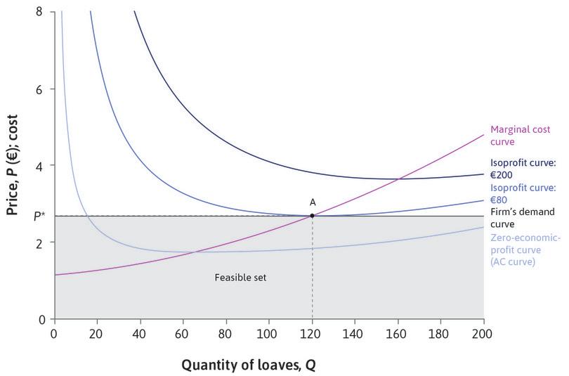
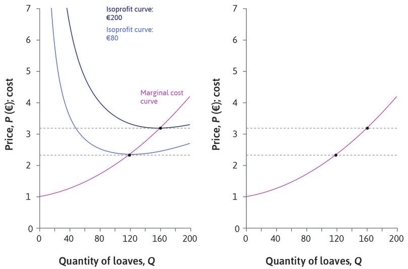
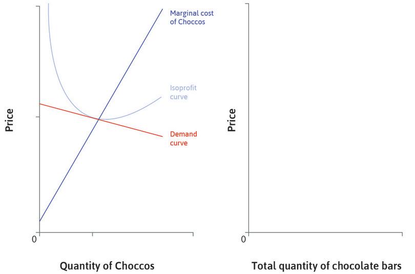
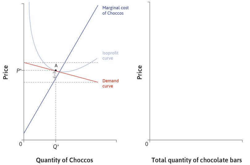
The marginal and average cost curves are drawn in Figure 8.5. As in Unit 7, costs include the opportunity cost of capital. If price were equal to average cost (P = AC), your economic profit would be zero. You, the owner, would obtain a normal return on your capital. So the average cost curve (the leftmost curve in Figure 8.5) is the zero-economic-profit curve. The isoprofit curves show price and quantity combinations at which you would receive higher levels of profit. As we explained in Unit 7, isoprofit curves slope downwards where price is above marginal cost, and upwards where price is below marginal cost, so the marginal cost curve passes through the lowest point on each isoprofit curve. If price is above marginal cost, total profits can remain unchanged only if a larger quantity is sold for a lower price. Similarly, if price is below marginal cost, total profits can remain unchanged only if a larger quantity is sold for a higher price.
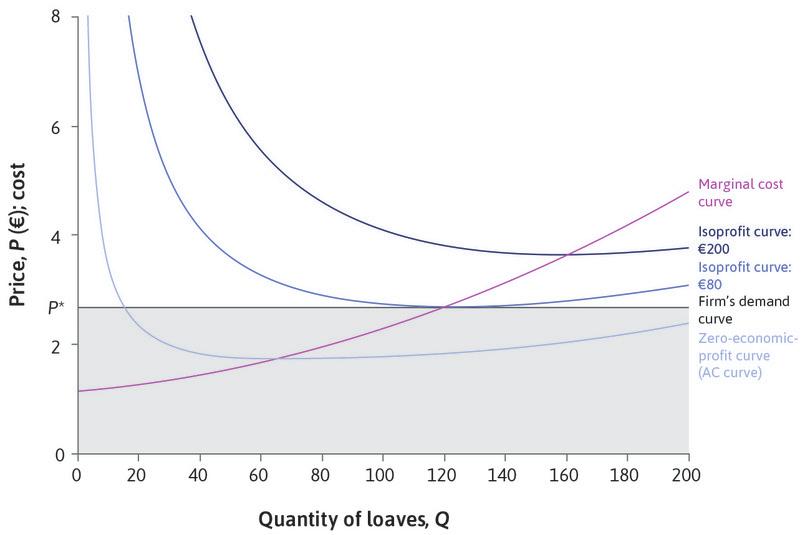
Figure 8.5 demonstrates how to make your decision. Like the firms in Unit 7, you face a constrained optimization problem. You want to find the point of maximum profit in your feasible set.
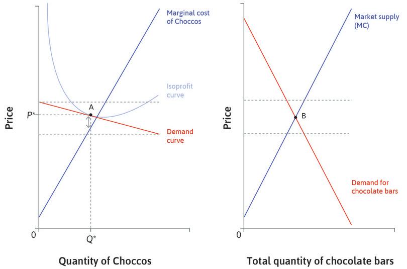
Because you are a price-taker, the feasible set is all points where price is less than or equal to €2.35, the market price. Your optimal choice is P* = €2.35 and Q* = 120, where the isoprofit curve is tangent to the feasible set. The problem looks similar to the one for Beautiful Cars in Unit 7, except that for a price-taker, the demand curve is completely flat. For your bakery, it is not the market demand curve in Figure 8.4 that affects your own demand, it is the price charged by your competitors. This is why the horizontal line at P* in Figure 8.5 is labelled as the firm’s demand curve. If you charge more than P*, your demand will be zero, but at P* or less you can sell as many loaves as you like.
Figure 8.5 illustrates a very important characteristic of price-taking firms. They choose to produce a quantity at which the marginal cost is equal to the market price (MC = P*). This is always true. For a price-taking firm, the demand curve for its own output is a horizontal line at the market price, so maximum profit is achieved at a point on the demand curve where the isoprofit curve is horizontal. And we know from Unit 7 that where isoprofit curves are horizontal, the price is equal to the marginal cost.
Another way to understand why a price-taking firm produces at the level of output where MC = P* is to think about what would happen to its profits if it deviated from this point. If the firm were to increase output to a level where MC > P*, the last unit would cost more than P* to make, so the firm would make a loss on this unit and could make higher profits by reducing output. If it were to produce where MC < P*, it could produce at least one more unit and sell it at a profit. Therefore it should raise output as far as the point where MC = P*. This is where profits are maximized.
Price-taking firm
A price-taking firm maximizes profit by choosing a quantity where the marginal cost is equal to the market price (MC = P*) and selling at the market price P*.
This is an important result that you should remember, but you need to be careful with it. When we make statements like ‘for a price-taking firm, price equals marginal cost’, we do not mean that the firm chooses a price equal to its marginal cost. Instead, we mean the opposite: the firm accepts the market price, and chooses its quantity so that the marginal cost is equal to that price.
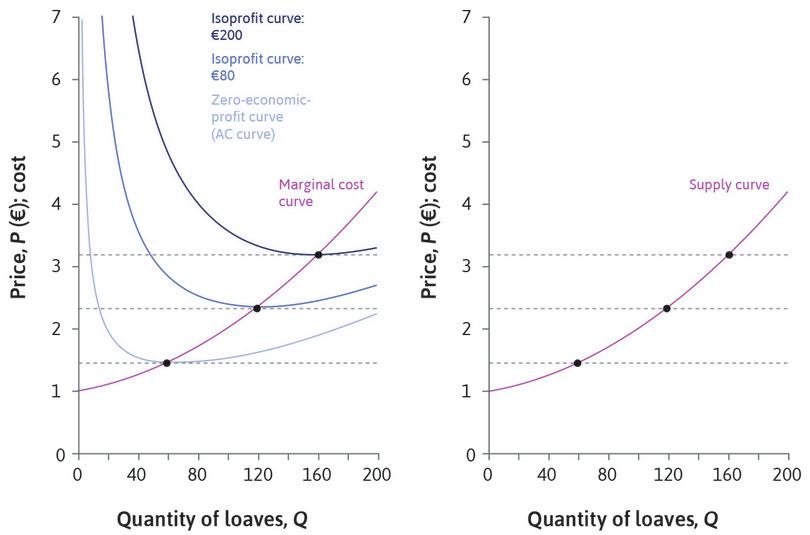
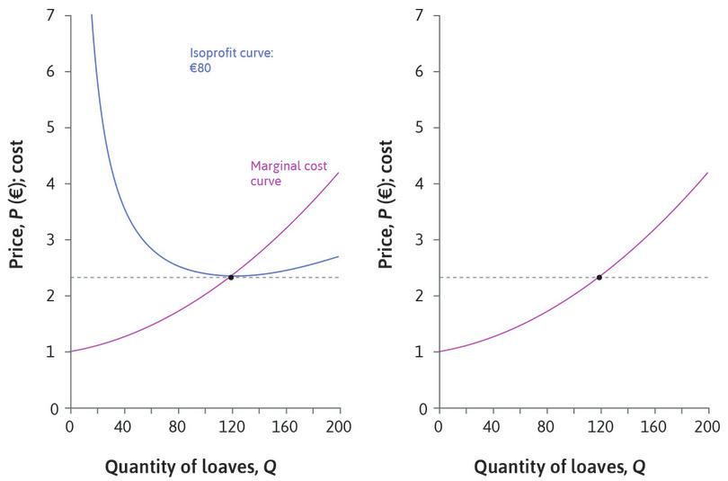
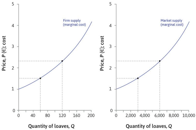
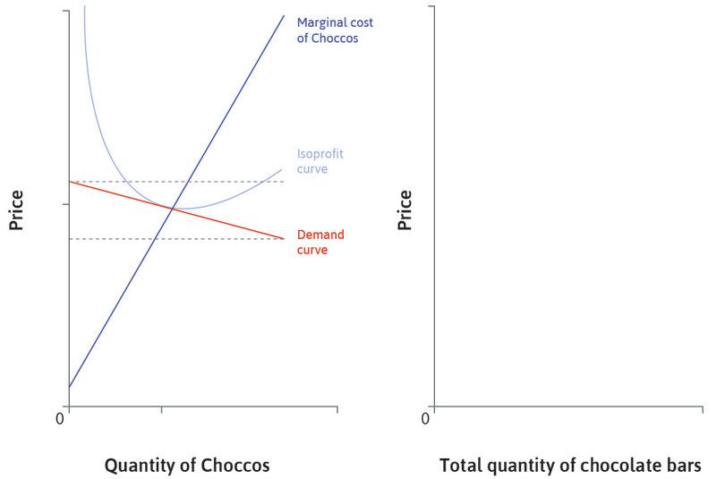
Put yourself in the position of the bakery owner again. What would you do if the market price changed? Figure 8.6 demonstrates that as prices change you would choose different points on the marginal cost curve.
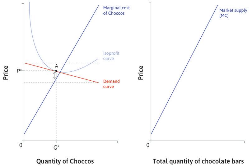
For a price-taking firm, the marginal cost curve is the supply curve: for each price it shows the profit-maximizing quantity—that is, the quantity that the firm will choose to supply.
Notice, however, that if the price fell below €1.52 you would be making a loss. The supply curve shows how many loaves you should produce to maximize profit, but when the price is this low, the economic profit is nevertheless negative. On the supply curve, you would be minimizing your loss. If this happened, you would have to decide whether it was worth continuing to produce bread. Your decision depends on what you expect to happen in the future:
- If you expect market conditions to remain bad, it might be best to sell up and leave the market—you could obtain a better return on your capital elsewhere.
- If you expect the price to rise soon, you might be willing to incur some short-term losses, and it might be worth continuing to produce bread if the revenue helped you to cover the costs of maintaining your premises and retaining staff.
Question 8.3 Choose the correct answer(s)
Figure 8.5 shows a price-taking bakery’s marginal and average cost curves, and its isoprofit curves. The market price for bread is P*= €2.35. Which of the following statements is correct?
- The firm’s demand curve is horizontal. Its supply curve is upward sloping.
- At €2.35 the firm maximizes profit at point A, where it supplies 120 loaves.
- At each price, the firm will choose a point on the highest isoprofit curve attainable, which will be a point on the marginal cost curve.
- At each price, the firm maximizes profit by choosing the corresponding quantity on the marginal cost curve. So the marginal cost curve is its supply curve.
8.4 Market supply and equilibrium
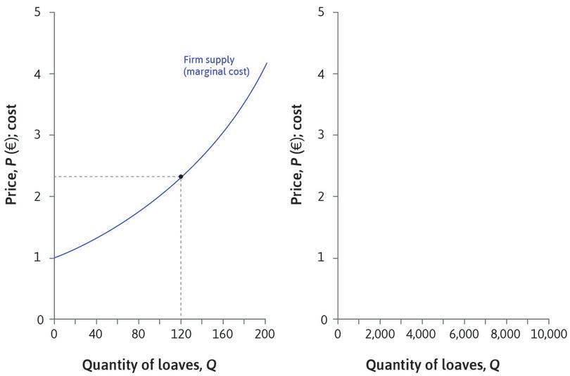
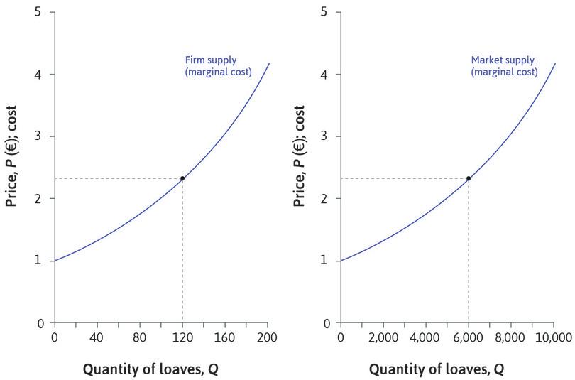
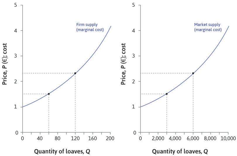
The market for bread in the city has many consumers and many bakeries. Let’s suppose there are 50 bakeries. Each one has a supply curve corresponding to its own marginal cost curve, so we know how much it will supply at any given market price. To find the market supply curve, we just add up the total amount that all the bakeries will supply at each price.
Figure 8.7 shows how this works if all the bakeries have the same cost functions. We work out how much one bakery would supply at a given price, then multiply by 50 to find total market supply at that price.
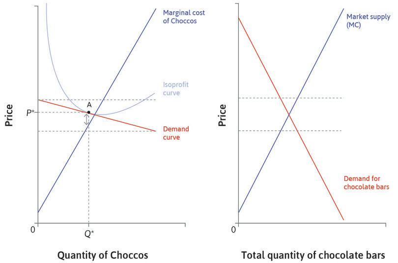
The market supply curve shows the total quantity that all the bakeries together would produce at any given price. It also represents the marginal cost of producing a loaf, just as the firm’s supply curve does. For example, if the market price is €2.75, total market supply is 7,000. For every bakery, the marginal cost—the cost of producing one more loaf—is €2.75. And that means that the cost of producing the 7,001st loaf in the market is €2.75, whichever firm produces it. So the market supply curve is the market’s marginal cost curve.
Leibniz: Market supply curve
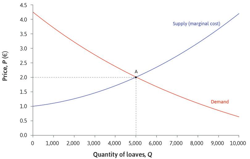
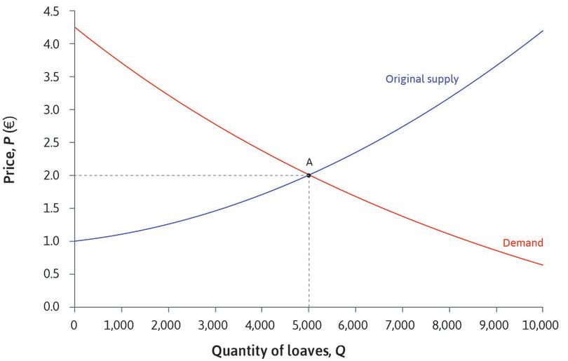
Now we know both the demand curve (Figure 8.4) and the supply curve (Figure 8.7) for the bread market as a whole. Figure 8.8 shows that the equilibrium price is exactly €2.00. At this price, the market clears: consumers demand 5,000 loaves per day, and firms supply 5,000 loaves per day.
Leibniz: Market equilibrium
In the market equilibrium, each bakery is producing on its marginal cost curve, at the point where its marginal cost is €2.00. If you look back to the isoprofit curves in Figure 8.6, you will see that the firm is above its average cost curve, the isoprofit curve where economic profits are zero. So the owners of the bakeries are receiving economic rents (profit in excess of normal profit). Whenever there are economic rents, there is an opportunity for someone to benefit by taking an action. In this case, we might expect the economic rents to attract other bakeries into the market. We will see presently how this would affect the market equilibrium.
Question 8.4 Choose the correct answer(s)
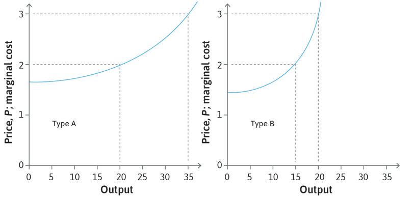
There are two different types of producers of a good in an industry where firms are price-takers. The marginal cost curves of the two types are given below:
Type A is more efficient than Type B: for example, as shown, at the output of 20 units, the Type A firms have a marginal cost of $2, as opposed to a marginal cost of $3 for the Type B firms. There are 10 Type A firms and 8 Type B firms in the market. Which of the following statements is correct?
- At $2, type A firms supply 20 units and type B firms supply 15 units. So the market supply is (10 × 20) + (8 × 15) = 320.
- At $3, type A firms supply 35 units and type B firms supply 20 units. So the market supply is (10 × 35) + (8 × 20) = 510.
- Both types will be producing at the marginal cost of $2. Therefore the market marginal cost is $2, irrespective of which firm produces the extra unit.
- The market’s marginal cost curve is its supply curve. We can calculate supply at each price as in (a) and (b).
8.5 Competitive equilibrium: Gains from trade, allocation, and distribution
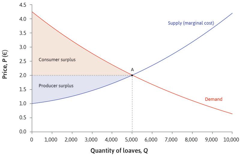
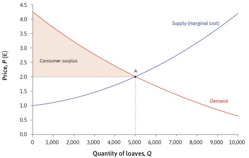
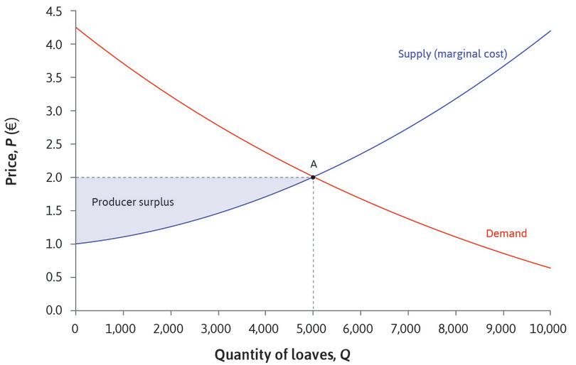
Buyers and sellers of bread voluntarily engage in trade because both benefit. Their mutual benefits from the equilibrium allocation can be measured by the consumer and producer surpluses introduced in Unit 7. Any buyer whose willingness to pay for a good is higher than the market price receives a surplus: the difference between the WTP and the price paid. Similarly, if the marginal cost of producing a good is below the market price, the producer receives a surplus. Figure 8.9a shows how to calculate the total surplus (the gains from trade) at the competitive equilibrium in the market for bread, in the same way as we did for the markets in Unit 7.
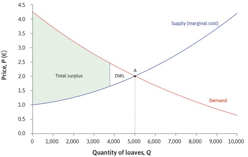
When the market for bread is in equilibrium with the quantity of loaves supplied equal to the quantity demanded, the total surplus is the area below the demand curve and above the supply curve.
Notice how the equilibrium allocation in this market differs from the allocation of a differentiated product, Beautiful Cars, in Unit 7. The equilibrium quantity of bread is at the point where the market supply curve, which is also the marginal cost curve, crosses the demand curve, and the total surplus is the whole of the area between the two curves. Figure 7.13 showed that in the market for Beautiful Cars, the manufacturer chooses to produce a quantity below the point where the marginal cost curve meets the demand curve, and the total surplus is lower than it would be at that point.
- deadweight loss
- A loss of total surplus relative to a Pareto-efficient allocation.
The competitive equilibrium allocation of bread has the property that the total surplus is maximized. Figure 8.9b shows that the surplus would be smaller if fewer than 5,000 loaves were produced. There would be consumers without bread who would be willing to pay more than the cost of producing another loaf, so there would be unexploited gains from trade. The total gains from trade in the market would be lower. We say there would be a deadweight loss equal to the triangle-shaped area. Producers would be missing out on potential profits, and some consumers would be unable to obtain the bread they were willing to pay for.
Leibniz: Gains from trade
And if more than 5,000 loaves were produced, the surplus on the extra loaves would be negative: they would cost more to make than consumers were willing to pay. (Is the exchange of gifts at Christmas a similar case of deadweight loss?)
Joel Waldfogel, an economist, gave his chosen discipline a bad name by suggesting that gift-giving at Christmas may result in a deadweight loss.4 If you receive a gift that is worth less to you than it cost the giver, you could argue that the surplus from the transaction is negative. Do you agree?5
At the equilibrium, all the potential gains from trade are exploited. This property—that the combined consumer and producer surplus is maximized at the point where supply equals demand—holds in general: if both buyers and sellers are price-takers, the equilibrium allocation maximizes the sum of the gains achieved by trading in the market, relative to the original allocation. We demonstrate this result in our Einstein at the end of this section.
Pareto efficiency
- Pareto efficient
- An allocation with the property that there is no alternative technically feasible allocation in which at least one person would be better off, and nobody worse off.
At the competitive equilibrium allocation in the bread market, it is not possible to make any of the consumers or firms better off (that is, to increase the surplus of any individual) without making at least one of them worse off. Provided that what happens in this market does not affect anyone other than the participating buyers and sellers, we can say that the equilibrium allocation is Pareto efficient.
Pareto efficiency follows from three assumptions we have made about the bread market.
Price-taking
The participants are price-takers. They have no market power. When a particular buyer trades with a particular seller, each of them knows that the other can find an alternative trading partner willing to trade at the market price. Sellers can’t raise the price because of competition from other sellers, and competition from other buyers prevents buyers from lowering it. Hence the suppliers will choose their output so that the marginal cost (the cost of the last unit produced) is equal to the market price.
In contrast, the producer of a differentiated good has bargaining power because it faces less competition: no one else produces an identical good. The firm uses its power to keep the price high, raising its own share of the surplus but lowering total surplus. The price is above marginal cost, so the allocation is Pareto inefficient.
A complete contract
The exchange of a loaf of bread for money is governed by a complete contract between buyer and seller. If you find there is no loaf of bread in the bag marked ‘bread’ when you get home, you can get your money back. Compare this with the incomplete employment contract in Unit 6, in which the firm can buy the worker’s time, but cannot be sure how much effort the worker will put in. We will see in Unit 9 that this leads to a Pareto-inefficient allocation in the labour market.
No effects on others
We have implicitly assumed that what happens in this market affects no one except the buyers and sellers. To assess Pareto efficiency, we need to consider everyone affected by the allocation. If, for example, the early morning activities of bakeries disrupt the sleep of local residents, then there are additional costs of bread production and we ought to take the costs to the bakeries’ neighbours into account too. Then, we may conclude that the equilibrium allocation is not Pareto efficient after all. We will investigate this type of problem in Unit 12.
Fairness
Remember from Unit 5 that there are two criteria for assessing an allocation: efficiency and fairness. Even if we think that the market allocation is Pareto efficient, we should not conclude that it is necessarily a desirable one. What can we say about fairness in the case of the bread market? We could examine the distribution of the gains from trade between producers and consumers: Figure 8.9a showed that both consumers and firms obtain a surplus, and in this example consumer surplus is slightly higher than producer surplus. You can see that this happens because the demand curve is relatively steep compared with the supply curve. Recall also from Unit 7 that a steep demand curve corresponds to a low elasticity of demand. Similarly, the slope of the supply curve corresponds to the elasticity of supply: in Figure 8.9a, demand is less elastic than supply.
In general, the distribution of the total surplus between consumers and producers depends on the relative elasticities of demand and supply.
We might also want to take into account the market participants’ standard of living. For example, if a poor student buys a book from a rich student, we might think that an outcome in which the buyer paid less than the market price (closer to the seller’s reservation price) would be better, because it would be fairer. Or, if the consumers in the bread market were exceptionally poor, we might decide that it would be better to pass a law setting a maximum bread price lower than €2.00 to achieve a fairer (although Pareto-inefficient) outcome.6 In Unit 11, we will look at the effect of regulating markets in this way.
The Pareto efficiency of a competitive equilibrium allocation is often interpreted as a powerful argument in favour of markets as a means of allocating resources. But we need to be careful not to exaggerate the value of this result:
- The allocation may not be Pareto efficient: We might not have taken everything into account.
- There are other important considerations: Fairness, for example.
- Price-takers are hard to find in real life: It is not as easy as you might think to find behaviour consistent with our simple model of the bread market (as we will see in Section 8.9).
- willingness to pay (WTP)
- An indicator of how much a person values a good, measured by the maximum amount he or she would pay to acquire a unit of the good. See also: willingness to accept.
- willingness to accept (WTA)
- The reservation price of a potential seller, who will be willing to sell a unit only for a price at least this high. See also: willingness to pay.
Exercise 8.3 Maximizing the surplus
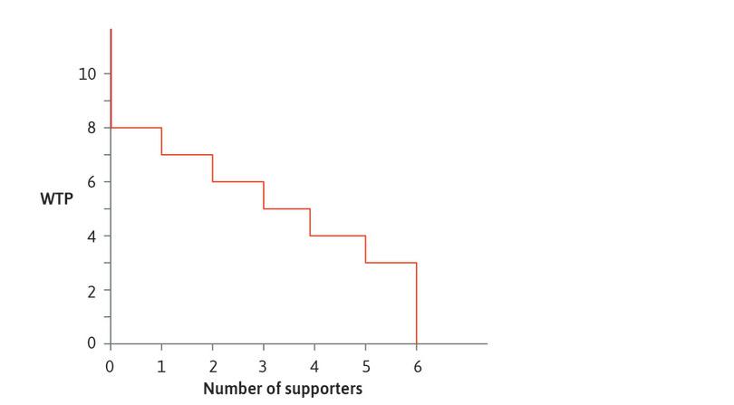
Consider a market for the tickets to a football match. Six supporters of the Blue team would like to buy tickets; their valuations of a ticket (their WTP) are 8, 7, 6, 5, 4, and 3. The diagram below shows the demand ‘curve’. Six supporters of the Red team already have tickets, for which their reservation prices (WTA) are 2, 3, 4, 5, 6, and 7.
- Draw the supply and demand ‘curves’ on a single diagram (Hint: the supply curve is also a step function, like the demand curve).
- Show that four trades take place in equilibrium.
- What is the equilibrium price?
- Calculate the consumer (buyer) surplus by adding up the surpluses of the four buyers who trade.
- Similarly calculate the producer (or seller) surplus.
- Hence, find the total surplus in equilibrium.
- Suppose that the market operates through bargaining between individual buyers and sellers. Find a way of matching the buyers and sellers so that more than four trades occur. (Hint: suppose the highest WTP buyer buys from the highest WTA seller.)
- In this case, work out the surplus from each trade.
- How does the total surplus in this case compare with the equilibrium surplus?
- Starting from the allocation of tickets you obtained through bargaining, in which at least five tickets are owned by Blue supporters, is there a way through further trade to make one of the supporters better off without making anyone worse off?
Exercise 8.4 Surplus and deadweight loss
- Sketch a diagram to illustrate the competitive market for bread, showing the equilibrium where 5,000 loaves are sold at a price of €2.00.
- Suppose that the bakeries get together to form a cartel. They agree to raise the price to €2.70, and jointly cut production to supply the number of loaves that consumers demand at that price. Shade the areas on your diagram to show the consumer surplus, producer surplus, and deadweight loss caused by the cartel.
- For what kinds of goods would you expect the supply curve to be highly elastic?
- Draw diagrams to illustrate how the share of the gains from trade obtained by producers depends on the elasticity of the supply curve.
Question 8.5 Choose the correct answer(s)
In Figure 8.9a, the market equilibrium output and price of the bread market is shown to be at (Q*, P*) = (5,000, €2). Suppose that the mayor decrees that bakeries must sell as much bread as consumers want, at a price of €1.50. Which of the following statements are correct?
- Producer surplus is lower, because the price is below marginal cost.
- Consumer surplus is higher, because the price of the first 5,000 loaves is lower, and for the additional loaves it is below the consumers’ WTP.
- The consumers benefit from the lower price, but producers lose because the price is below marginal cost.
- There is a deadweight loss, equal to the area of the triangle between the supply and demand curves to the right of equilibrium.
Question 8.6 Choose the correct answer(s)
Which of the following statements about a competitive equilibrium allocation are correct?
- The allocation maximizes the total surplus, but the does not mean it is best for everyone in the market—for example, we may think it is unfair.
- This must be true, since the allocation maximizes the total surplus.
- The equilibrium allocation may not be Pareto efficient if it affects someone other than the buyers or sellers.
- This is a general property of competitive equilibrium.
Einstein Total surplus and WTP
However the market works, and whatever prices are paid, we can calculate the consumer surplus by adding together the differences between WTP and price paid for all the people who buy, and the producer surplus by adding together the difference between price received and marginal cost of every unit of output:
Then when we calculate the total surplus, the prices paid and received cancel out:
When buyers and sellers are price-takers, and the price equalizes supply and demand, the total surplus is as high as possible, because the consumers with the highest WTPs buy the product and the units of output with the lowest marginal costs are sold. Every trade involves a buyer with a higher WTP than the seller’s reservation value, so the surplus would go down if we omitted any of them. And if we tried to include any more units of output in this calculation, the surplus would also go down because the WTPs would be lower than the MCs.
8.6 Changes in supply and demand
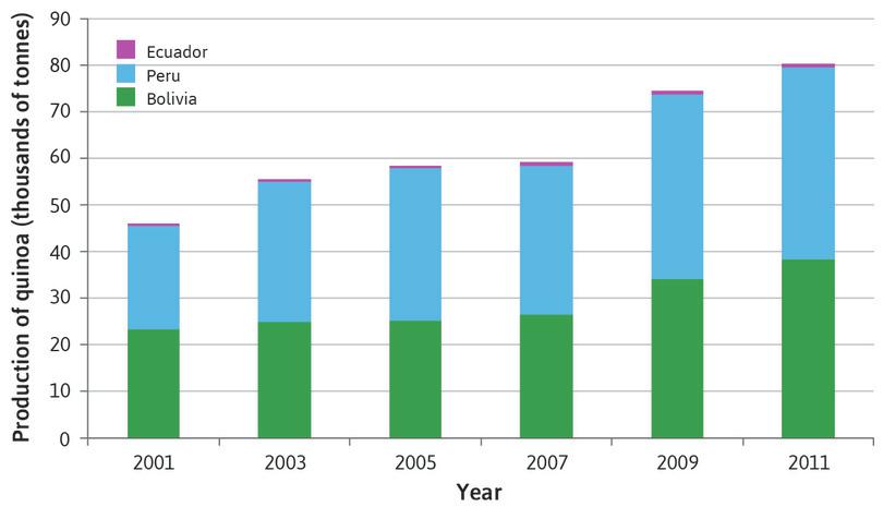
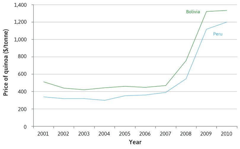
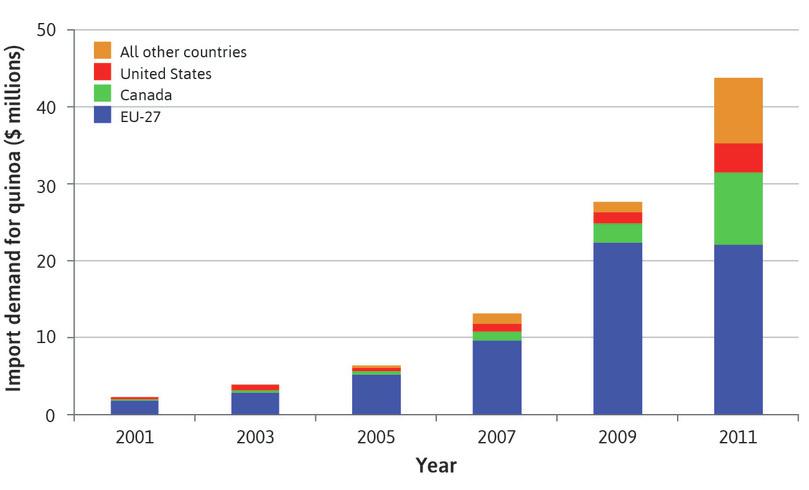
Quinoa is a cereal crop grown on the Altiplano, a high barren plateau in the Andes of South America. It is a traditional staple food in Peru and Bolivia. In recent years, as its nutritional properties have become known, there has been a huge increase in demand from richer, health-conscious consumers in Europe and North America. Figures 8.10a–c show how the market changed. You can see in Figures 8.10a and 8.10b that between 2001 and 2011, the price of quinoa trebled and production almost doubled. Figure 8.10c indicates the strength of the increase in demand: spending on imports of quinoa rose from just $2.4 million to $43.7 million in 10 years.
Jose Daniel Reyes and Julia Oliver. ‘Quinoa: The Little Cereal That Could’. The Trade Post. 22 November 2013. Underlying data from Food and Agriculture Organization of the United Nations. FAOSTAT Database.
For the producer countries these changes are a mixed blessing. While their staple food has become expensive for poor consumers, farmers—who are amongst the poorest—are benefiting from the boom in export sales. Other countries are now investigating whether quinoa can be grown in different climates, and France and the US have become substantial producers.
How can we explain the rapid increase in the price of quinoa? In this section, we look at the effects of changes in demand and supply in our simple examples of books and bread. At the end of this section you can apply the analysis to the real-world case of quinoa.
An increase in demand
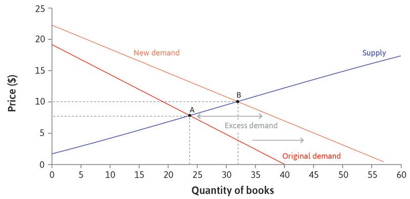
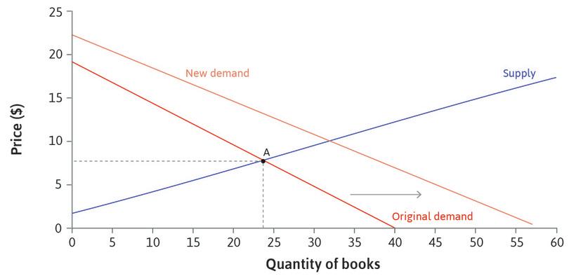
In the market for second-hand textbooks, demand comes from new students enrolling on the course, and supply comes from students who took the course in the previous year. In Figure 8.11 we have plotted supply and demand for textbooks when the number of students enrolling remains stable at 40 per year. The equilibrium price is $8 and 24 books are sold, as shown by point A. Suppose that in one year the course became more popular. Figure 8.11 shows what would happen.
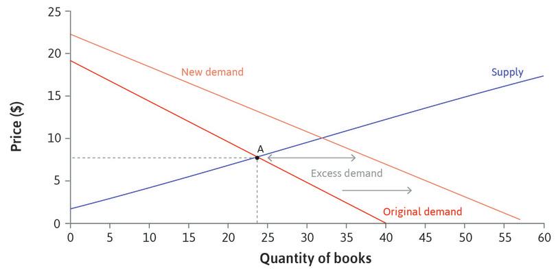
The increase in demand leads to a new equilibrium, in which 32 books are sold for $10 each. At the original price, there would be excess demand and sellers would want to raise their prices. At the new equilibrium, both price and quantity are higher. Some students who would not have sold their books at $8 will now sell at a higher price. Notice, however, that although demand has increased, not all the students who would have bought at $8 will purchase the book at the new equilibrium: those with WTP between $8 and $10 no longer want to buy.
When we say ‘increase in demand’, it’s important to be careful about exactly what we mean:
- Demand is higher at each possible price, so the demand curve has shifted.
- In response to this shift there is a change in the price.
- This leads to an increase in the quantity supplied.
- This change is a movement along the supply curve.
- But the supply curve itself has not shifted (the number of sellers and their reserve prices have not changed), so we do not call this ‘an increase in supply’.
After an increase in demand, the equilibrium quantity rises, but so does the price. You can see in Figure 8.11 that the steeper (more inelastic) the supply curve, the higher the price will rise and the lower the quantity will increase. If the supply curve is quite flat (elastic), then the price rise will be smaller and the quantity sold will be more responsive to the demand shock.
An increase in supply due to improved productivity
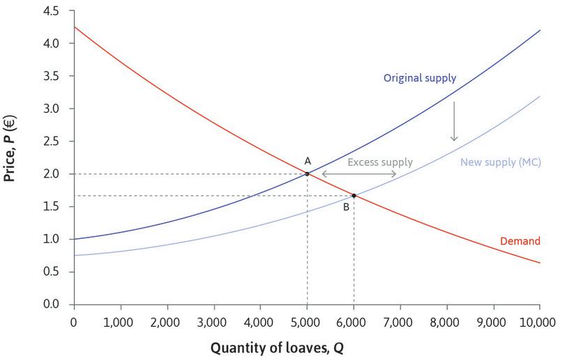
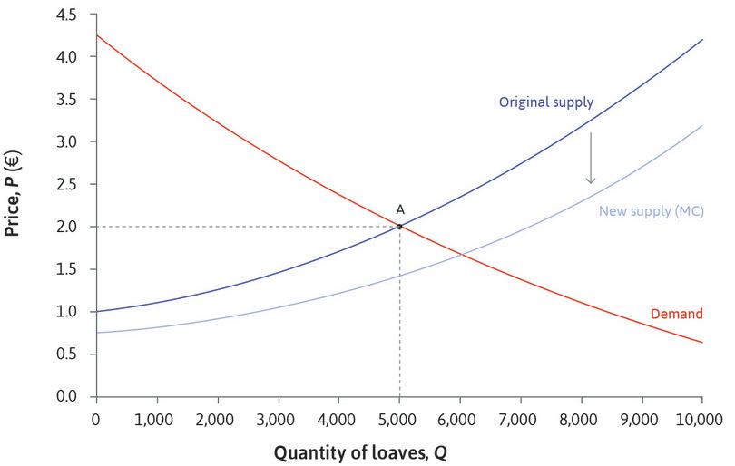
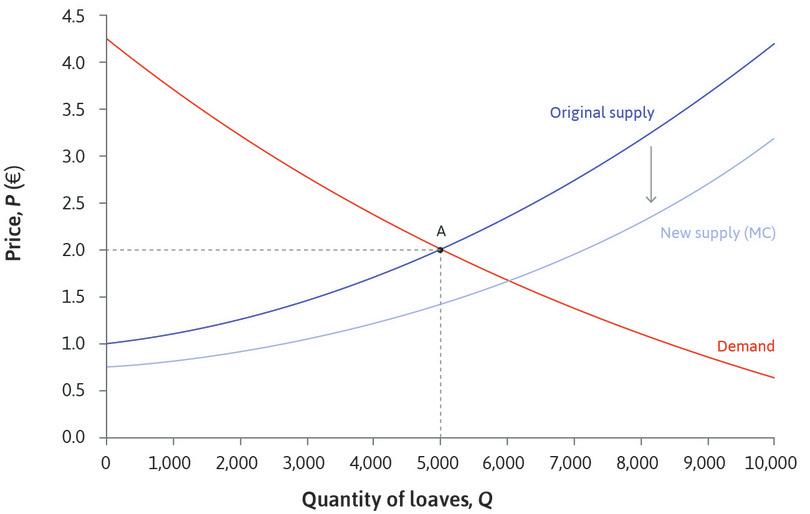
In contrast, as an example of an increase in supply, think again about the market for bread in one city. Remember that the supply curve represents the marginal cost of producing bread. Suppose that bakeries discover a new technique that allows each worker to make bread more quickly. This will lead to a fall in the marginal cost of a loaf at each level of output. In other words, the marginal cost curve of each bakery shifts down.
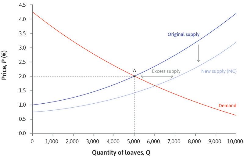
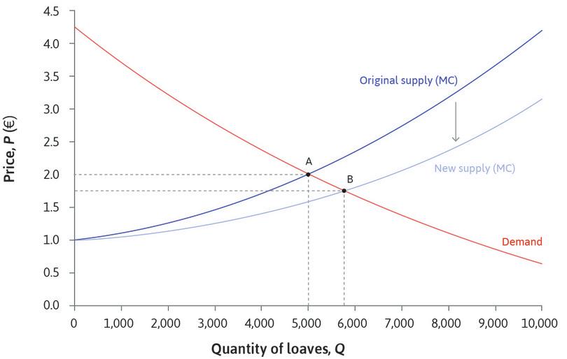
Figure 8.12 shows the original supply and demand curves for the bakeries. When the MC curve of each bakery shifts down, so does the market supply curve for bread. Look at Figure 8.12 to see what happens next.
The improvement in the technology of breadmaking leads to:
- an increase in supply
- a fall in the price of bread
- a rise in the quantity sold
Leibniz: Shifts in demand and supply
As in the example of an increase in demand, an adjustment of prices is needed to bring the market into equilibrium. Such shifts in supply and demand are often referred to as shocks in economic analysis. We start by specifying an economic model and find the equilibrium. Then we look at how the equilibrium changes when something changes—the model receives a shock. The shock is called exogenous because our model doesn’t explain why it happened: the model shows the consequences, not the causes.
- shock
- An exogenous change in some of the fundamental data used in a model.
- exogenous
- Coming from outside the model rather than being produced by the workings of the model itself. See also: endogenous.
An increase in supply: More bakeries enter the market
Another reason for a change in market supply is the entry of more firms or the exit of existing firms. We analysed the equilibrium of the bread market in the case when there were 50 bakeries in the city. Remember from Section 8.4 that at the equilibrium price of €2, each bakery is on an isoprofit curve above the average cost curve. If economic profits are greater than zero, firms are receiving an economic rent, so other firms might want to invest in the baking business.
- costs of entry
- Startup costs that would be incurred when a seller enters a market or an industry. These would usually include the cost of acquiring and equipping new premises, research and development, the necessary patents, and the cost of finding and hiring staff.
Since there is an opportunity for making greater than normal profit by selling bread in the city, new bakeries may decide to enter the market. There will be some costs of entry, for example, acquiring and equipping the premises, but provided these are not too high (or if premises and equipment can be easily sold if the venture doesn’t work out) it will be worthwhile to do so.
Remember that we find the market supply curve by adding up the amounts of bread supplied by each firm, at each price. When more bakeries have entered, more bread will be supplied at each price level. Although the reason for the supply increase is different from the previous one, the effect on the market equilibrium is the same: a fall in price and a rise in bread sales. Figure 8.13 shows the effects on equilibrium. The bakeries once again start off at point A, selling 5,000 loaves of bread for €2. The entry of new firms shifts the supply curve outwards. There is more bread for sale at each price, so at the original price there would be excess supply. The new equilibrium is at point B with a lower price and higher bread sales.
The entry of new firms is unlikely to be welcomed by the existing bakeries. Their costs have not changed, but the market price has fallen to €1.75, so they must be making less profit than before. As we will see in Unit 11, the entry of new firms may eventually drive economic profits to zero, eliminating rents altogether.
Exercise 8.5 The market for quinoa
Consider again the market for quinoa. The changes shown in Figures 8.10a–c can be analysed as shifts in demand and supply.
- Suppose there was an unexpected increase in demand for quinoa in the early 2000s (a shift in the demand curve). What would you expect to happen to the price and quantity initially?
- Assuming that demand continued to rise over the next few years, how do you think farmers responded?
- Why did the price stay constant until 2007?
- How could you account for the rapid price rise in 2008 and 2009?
- Would you expect the price to fall eventually to its original level?
Exercise 8.6 Prices, shocks, and revolutions
Historians usually attribute the wave of revolutions in Europe in 1848 to long-term socioeconomic factors and a surge of radical ideas. But a poor wheat harvest in 1845 lead to food shortages and sharp price rises, which may have contributed to these sudden changes.7
The table shows the average and peak prices of wheat from 1838 to 1845, relative to silver. There are three groups of countries: those where violent revolutions took place, those where constitutional change took place without widespread violence, and those where no revolution occurred.
- Explain, using supply and demand curves, how a poor wheat harvest could lead to price rises and food shortages.
- Find a way to present the data to show that the size of the price shock, rather than the price level, is associated with the likelihood of revolution.
- Do you think this is a plausible explanation for the revolutions that occurred?
- A journalist suggests that similar factors played a part in the Arab Spring in 2010. Read the post. What do you think of this hypothesis?
Avg. price 1838–45 Max. price 1845–48 Violent revolution 1848 Austria 52.9 104.0 Baden 77.0 136.6 Bavaria 70.0 127.3 Bohemia 61.5 101.2 France 93.8 149.2 Hamburg 67.1 108.7 Hessedarmstadt 76.7 119.7 Hungary 39.0 92.3 Lombardy 88.3 119.9 Mecklenburgschwerin 72.9 110.9 Papal states 74.0 105.1 Prussia 71.2 110.7 Saxony 73.3 125.2 Switzerland 87.9 146.7 Württemberg 75.9 128.7 Immediate constitutional change 1848 Belguim 93.8 140.1 Bremen 76.1 109.5 Brunswick 62.3 100.3 Denmark 66.3 81.5 Netherlands 82.6 136.0 Oldenburg 52.1 79.3 No revolution 1848 England 115.3 134.7 Finland 73.6 73.7 Norway 89.3 119.7 Russia 50.7 44.1 Spain 105.3 141.3 Sweden 75.8 81.4 Berger, Helge, and Mark Spoerer. 2001. ‘Economic Crises and the European Revolutions of 1848.’ The Journal of Economic History 61 (2): pp. 293–326.
Question 8.7 Choose the correct answer(s)
Figure 8.8 shows the equilibrium of the bread market to be 5,000 loaves per day at price €2. A year later, we find that the market equilibrium price has fallen to €1.50. What can we conclude?
- This is not the only possible cause of a fall in price.
- This is not the only possible cause of a fall in price.
- A downward shift in either curve would cause the price to fall. If we knew whether output had increased or decreased, we could determine which curve had shifted.
- At the market equilibrium price, there is no excess demand or supply.
Question 8.8 Choose the correct answer(s)
Which of the following statements are correct?
- If mortgage borrowing becomes cheaper, more people will want to buy houses at each house price.
- A launch of a substitute would decrease demand, shifting the demand curve down.
- The quantity of oil demanded would increase by moving along the demand curve; the curve itself would not move.
- The marginal cost of producing plastics would fall, so the supply curve would shift down.
8.7 The effects of taxes
Governments can use taxation to raise revenue (to finance government spending, or redistribute resources) or to affect the allocation of goods and services in other ways, perhaps because the government considers a particular good to be harmful. The supply and demand model is a useful tool for analysing the effects of taxation.
Using taxes to raise revenue
Raising revenue through taxation has a long history (see Unit 22). Take the taxation of salt, for example. For most of history, salt was used all over the world as a preservative, allowing food to be stored, transported, and traded. The ancient Chinese advocated taxing salt, since people needed it, however high the price. Salt taxes were an effective but often resented tool used by ruling elites in ancient India and medieval kings. Resentment of high salt taxes played an important part in the French Revolution, and Gandhi led protests against the salt tax imposed by the British in India.
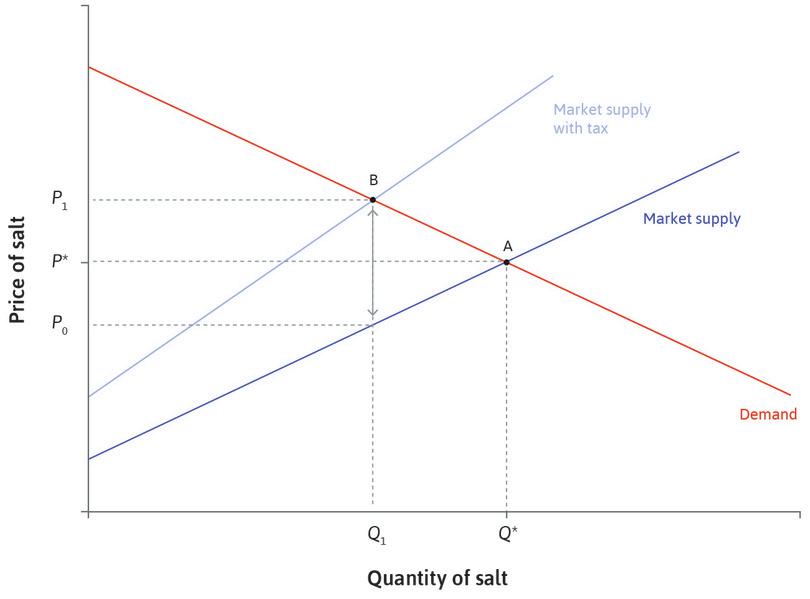
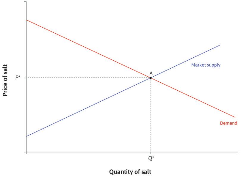
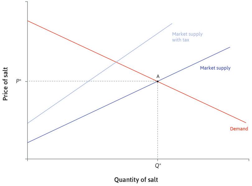
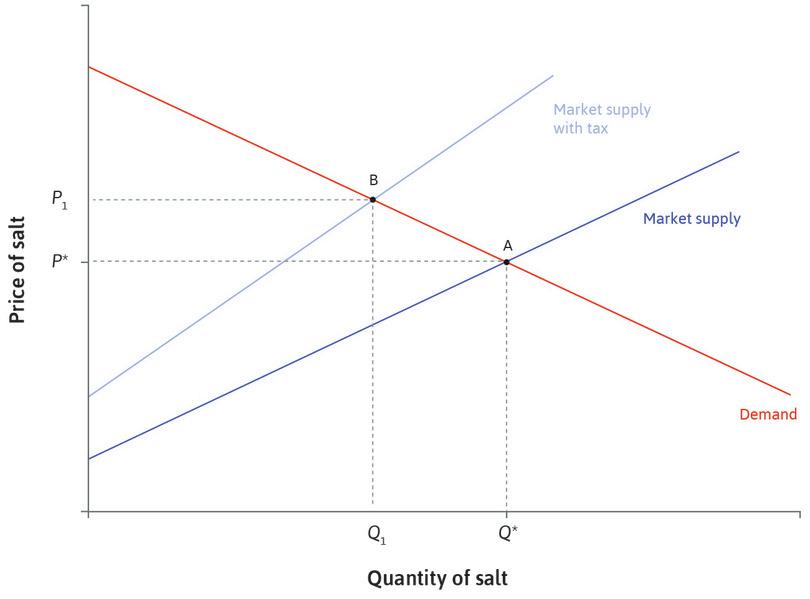
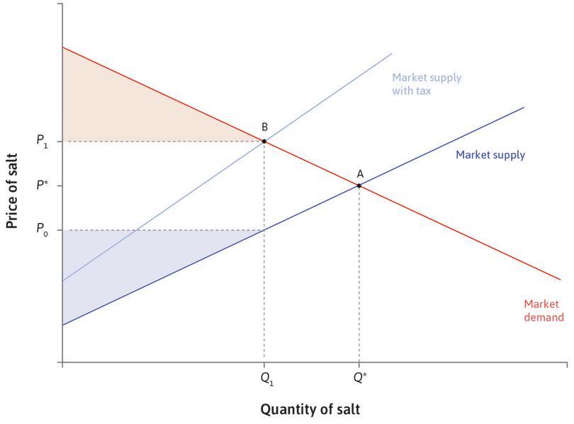
Figure 8.14 illustrates how a salt tax might work. Initially the market equilibrium is at point A: the price is P* and the quantity of salt traded is Q*. Suppose that a sales tax of 30% is imposed on the price of salt, to be paid to the government by the suppliers. If suppliers have to pay a 30% tax, their marginal cost of supplying each unit of salt increases by 30%. So the supply curve shifts: the price is 30% higher at each quantity.
The new equilibrium is at point B, where a lower quantity of salt is traded. Although the consumer price has risen, note that it is not 30% higher than before. The price paid by consumers, P1, is 30% higher than the price received by the suppliers (net of the tax), which is P0. Suppliers receive a lower price than before, they produce less, and their profits will be lower. This illustrates an important feature of taxes: it is not necessarily the taxpayer who feels its main effect. In this case, although the suppliers pay the tax, the tax incidence falls partly on consumers and partly on producers.
- tax incidence
- The effect of a tax on the welfare of buyers, sellers, or both.
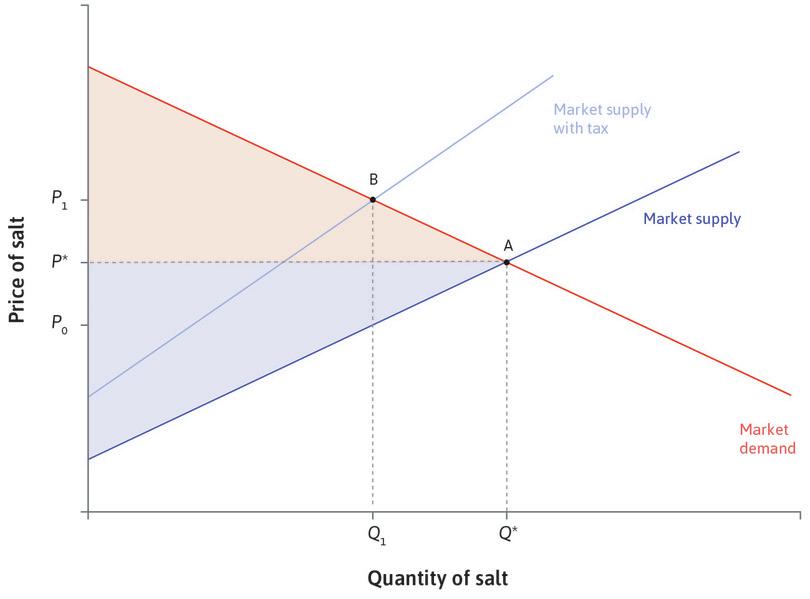
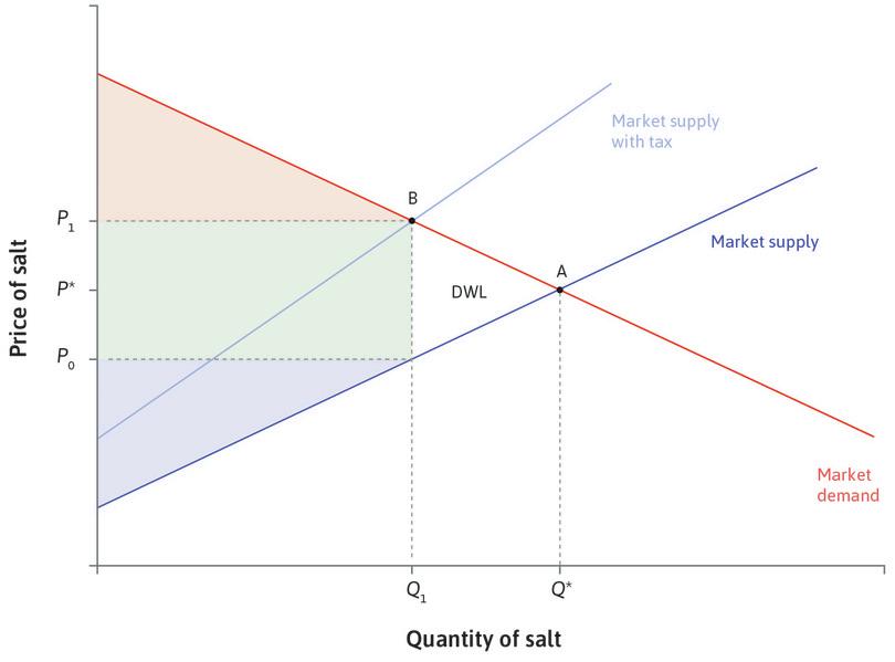
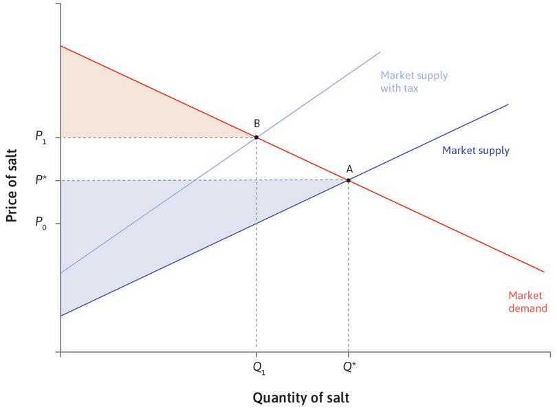
Figure 8.15 shows the effect of the tax on consumer and producer surplus:
- Consumer surplus falls: Consumers pay a higher price, and buy less salt.
- Producer surplus falls: They produce less and receive a lower net price.
- Total surplus is lower: Even taking account of the tax revenue received by the government, the tax causes a deadweight loss.
When the salt tax is imposed, the total surplus from trade in the salt market is given by:
Since the quantity of salt traded is no longer at the level that maximizes gains from trade, the tax has led to a deadweight loss.
In general, taxes change prices, and prices change buyers’ and sellers’ decisions, which can cause deadweight loss. To raise as much revenue as possible, the government would prefer to tax a good for which demand is not very responsive to price, so that the fall in quantity traded is quite small—that is to say, a good with a low elasticity of demand. That is why the ancient Chinese recommended taxing salt.
We can think of the total surplus as a measure of the welfare of society as a whole (provided that the tax revenue is used for the benefit of society). So there is a second reason for a government that cares about welfare to prefer taxing goods with low elasticity of demand—the loss of total surplus will be lower. The overall effect of the tax depends on what the government does with the revenues that it collects:
- The government spends the revenue on goods and services that enhance the wellbeing of the population: Then the tax and resulting expenditure may enhance public welfare—even though it reduces the surplus in the particular market that is taxed.
- The government spends the revenues on an activity that does not contribute to wellbeing: Then the lost consumer surplus is just a reduction in the living standards of the population.
Therefore, taxes can improve or reduce overall welfare. The most that we can say is that taxing a good whose demand is inelastic is an efficient way to transfer the surplus from consumers to the government.
The government’s power to levy taxes is a bit like the price-setting power of a firm that sells a differentiated good. It uses its power to raise the price and collect revenue, while reducing the quantity sold. Its ability to levy taxes depends on the institutions it can use to enforce and collect them.
One reason for the use of salt taxes in earlier times was that it was relatively easy for a powerful ruler to take full control of salt production, in some cases as a monopolist. In the notorious case of the French salt tax, the monarchy not only controlled all salt production; it also forced its subjects to buy up to 7 kg of salt each per year.
In March and April 1930, the artificially high price of salt in British colonial India provoked one of the defining moments of the Indian independence movement: Mahatma Gandhi’s salt march to acquire salt from the Indian ocean. Similarly, in what came to be called the Boston tea party, in 1773 American colonists objecting to a British colonial tax on tea dumped a cargo of tea into the Boston harbour.
Resistance to taxes on inelastic goods arises for the very reason they are imposed: they are difficult to escape!
In many modern economies the institutions for tax collection are well-established, usually with democratic consent. Provided that citizens believe taxes have been implemented fairly, using them to raise revenue is accepted as a necessary part of social and economic policy. We will now look at another reason why governments may decide to levy taxes.
Using taxes to change behaviour
Policymakers in many countries are interested in the idea of using taxes to deter consumption of unhealthy foods with the objective of improving public health and tackling the obesity epidemic. In Unit 7, we looked at some data and estimates of demand elasticities for food products in the US, which help to predict how higher prices might affect people’s diets there. Some countries have already introduced food taxes. Several, including France, Norway, Mexico, Samoa, and Fiji, tax sweetened drinks. Hungary’s ‘chips tax’ is aimed at products carrying proven health risks, particularly those with high sugar or salt content. In 2011, the Danish government introduced a tax on products with high saturated fat content.8
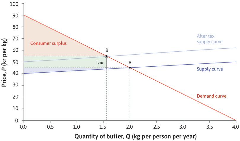
The level of the Danish tax was 16 Danish kroner (kr) per kilogram of saturated fat, corresponding to 10.4 kr per kg of butter. Note that this was a specific tax, levied as a fixed amount per unit of butter. A tax like the one we analysed for salt, levied as a percentage of the price, is known as an ad valorem tax. According to a study of the Danish fat tax, it corresponded to about 22% of the average butter price in the year before the tax. The study found that it reduced the consumption of butter and related products (butter blends, margarine, and oil) by between 15% and 20%. We can illustrate the effects in the same way as we did for the salt tax, using the supply and demand model (we are assuming here that butter retailers are price-takers).
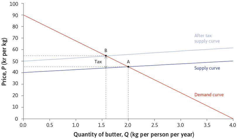
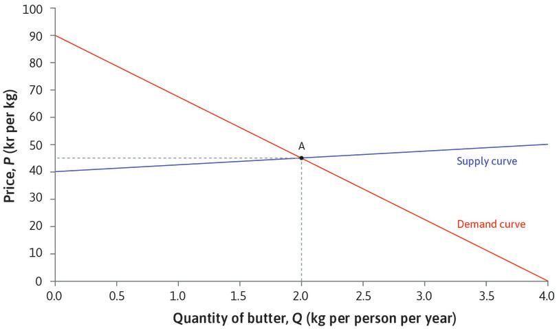
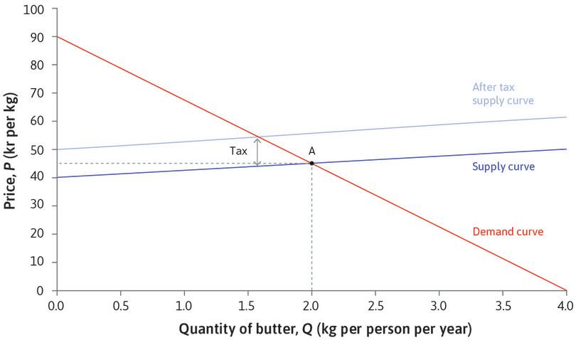
Figure 8.16 shows a demand curve for butter, measured in kilograms per person per year. The numbers correspond approximately to Denmark’s experience. We have drawn the supply curve for butter as almost flat, on the assumption that the marginal cost of butter for retailers does not change very much as quantity varies. The initial equilibrium is at point A, where the price of butter is 45 kr per kg, and each person consumes 2 kg of butter per year.
A tax of 10 kr per kg shifts the supply curve upwards and leads to a rise in price to 54 kr, and a fall in consumption to 1.6 kg. The consumer price rises by 9 kr—almost the full amount of the tax—and the suppliers’ net revenue per kg of butter falls to 44 kr. In this case, although suppliers pay the tax, the tax incidence is felt mainly by consumers. Of the 10 kr tax per kg, the consumer effectively pays 9 kr, while the supplier or producer pays 1 kr. So the price received by the retailers, net of tax, is only 1 kr lower.
Figure 8.17 shows what happens to consumer and producer surplus as a result of the fat tax.
Again, both consumer and producer surpluses fall. The area of the green rectangle represents the tax revenue: with a tax of 10 kr per kg and equilibrium sales of 1.6 kg per person, tax revenue is 10 × 1.6 = 16 kr per person per year.
How effective was the fat tax policy? For a full evaluation of the effect on health we should look at all the foods taxed, and take into account the cross-price effects—the changes in consumption of other foods caused by the tax. The study of the Danish tax also allowed for the possibility that some retailers are not price-takers. Nevertheless, Figures 8.16 and 8.17 illustrate some important implications of the tax:
- Consumption of butter products fell: In this case by 20%. You can see this in Figure 8.16. In this respect, the policy was successful.
- There was a large fall in surplus, especially consumer surplus: You can see this in Figure 8.17. But recall that the government’s aim when it implemented the fat tax policy was not to raise revenue, but rather to reduce quantity. So the fall in consumer surplus was inevitable. The loss of surplus caused by a tax is a deadweight loss, which sounds negative. But in this case the policymaker might see it as a gain if the ‘good’, butter, is considered ‘bad’ for consumers.
One aspect of taxation not illustrated in our supply and demand analysis is the cost of collecting it. Although the Danish fat tax successfully reduced fat consumption, the government abolished it after only 15 months because of the administrative burden it placed on firms. Any taxation system requires effective mechanisms for tax collection, and designing taxes that are simple to administer (and difficult to avoid) is an important goal of tax policy. Policymakers who want to introduce food taxes will need to find ways of minimizing administrative costs. But since the costs cannot be eliminated, they will also need to consider whether the health gain (and reduction of costs of bad health) will be sufficient to offset them.
Exercise 8.7 The deadweight loss of the butter tax
Food taxes such as the ones discussed here and in Unit 7 are often intended to shift consumption towards a healthier diet, but give rise to deadweight loss.
Why do you think a policymaker and a consumer might interpret this deadweight loss differently?
Question 8.9 Choose the correct answer(s)
Figure 8.14 shows the demand and supply curves for salt, and the shift in the supply curve due to the implementation of a 30% tax on the price of salt. Which of the following statements are correct?
- In the post-tax equilibrium, the consumers pay P₁ and the producers receive P0.
- The government’s tax revenue is (P1 – P0) × Q1.
- This is the area of the triangle between the supply and demand curves, below AB.
- This is the area of the trapezium between the horizontal dotted lines through A and B.
Question 8.10 Choose the correct answer(s)
Figure 8.17 shows the effect of a tax intended to reduce the consumption of butter. The before-tax equilibrium is at A = (2.0 kg, 45 kr) and the after-tax equilibrium is at B = (1.6 kg, 54 kr). The tax imposed is 10 kr per kg of butter. Which of the following statements is correct?
- The producers receive the price 54 – 10 = 44 kr per kg.
- If the supply curve were less elastic, the policy would be less effective—butter consumption would not fall as much.
- The elastic supply curve means that the price paid by consumers changes much more than the price received by producers.
- The calculation gives the deadweight loss, not the loss of consumer surplus.
8.8 The model of perfect competition
Perfect competition
A hypothetical market in which:
- The good or service being exchanged is homogeneous (it does not differ from one seller to another).
- There are large numbers of potential buyers and sellers of the good, each acting independently of the others.
- Buyers and sellers can readily know the prices at which other buyers and sellers are exchanging the good.
To apply the model of supply and demand, we have assumed throughout this unit that buyers and sellers are price-takers. In what kinds of markets would we expect to see price-taking on both sides? To generate competition between sellers, and force sellers to act as price-takers, we need:
- Many undifferentiated sellers: As Marshall discussed, there must be many sellers, all selling identical goods. If their goods were differentiated, then each one would have some market power.
- Sellers must act independently: If they act as a cartel, for example, they are not price-takers—they can jointly choose the price.
- Many buyers all wanting to buy the good: Each of them will choose whichever seller has the lowest price.
- Buyers know the sellers’ prices: If they do not, they cannot choose the lowest one.
Similarly, buyers must force each other to be price-takers:
- There must be many buyers, competing with each other: Then sellers have no reason to sell to someone who would pay less than everyone else.
- perfectly competitive equilibrium
- Such an equilibrium occurs in a model in which all buyers and sellers are price-takers. In this equilibrium, all transactions take place at a single price. This is known as the law of one price. At that price, the amount supplied equals the amount demanded: the market clears. No buyer or seller can benefit by altering the price they are demanding or offering. They are both price-takers. All potential gains from trade are realized. See also: law of one price.
A market with all of these properties is described as perfectly competitive. We can predict that the equilibrium in such a market will be a competitive equilibrium—so it will have the following characteristics:
- law of one price
- Holds when a good is traded at the same price across all buyers and sellers. If a good were sold at different prices in different places, a trader could buy it cheaply in one place and sell it at a higher price in another. See also: arbitrage.
- gains from exchange
- The benefits that each party gains from a transaction compared to how they would have fared without the exchange. Also known as: gains from trade. See also: economic rent.
- All transactions take place at a single price: This is known as the law of one price.
- At that price, the amount supplied equals the amount demanded: the market clears.
- No buyer or seller can benefit by altering the price they are demanding or offering. They are all price-takers.
- All potential gains from trade are realized.
Léon Walras, a ninteenth-century French economist, built a mathematical model of an economy in which all buyers and sellers are price-takers, which has been influential in how many economists think about markets.
Great economists Léon Walras
Léon Walras (1834–1910) was a founder of the neoclassical school of economics. He was an indifferent student, and twice failed the entrance exam to the École Polytechnique in Paris, one of the most prestigious universities in his native France. He studied engineering at the School of Mines instead. Eventually his father, an economist, convinced him to take up the challenge of making economics into a science.
The pure economic science to which he aspired was the study of relationships among things, not people, and he had notable success in eliminating human relationships from his modelling. ‘The pure theory of economics,’ he wrote, ‘resembles the physico-mathematical sciences in every respect.’
His device for simplifying the economy so that it could be expressed mathematically was to represent interactions among economic agents as if they were relationships among inputs and outputs, and to focus entirely on the economy in equilibrium. In the process the entrepreneur, a key actor in wealth creation from the Industrial Revolution to today, simply disappeared from Walrasian economics:
Assuming equilibrium, we may even go so far as to abstract from entrepreneurs and simply consider the productive services as being, in a certain sense, exchanged directly for one another … (Elements of Theoretical Economics, 1874)9
Walras represented basic economic relationships as equations, which he used to study the workings of an entire economy composed of many interlinked markets. Prior to Walras, most economists had considered these markets in isolation: they would have studied, for example, how the price of textiles is determined on the cloth market, or land rents on the land market.
A century before Walras, a group of French economists called the physiocrats had studied the circulation of goods throughout the economy, as if the flow of goods from one sector to another in the economy was comparable to the circulation of blood in the human body (one of the leading physiocrats was a medical doctor). But the physiocrats’ model was little more than a metaphor that drew attention to the interconnectedness of markets.
Walras used mathematics, rather than medical analogies, to create what is now called general equilibrium theory, a mathematical model of an entire economy in which all buyers and sellers act as price-takers and supply equals demand in all markets. Walras’ work was the basis of the proof, much later, of the invisible hand theorem, giving the conditions under which such an equilibrium is Pareto efficient. The invisible hand game in Unit 4 is an example of the conditions in which the pursuit of self-interest can benefit everyone.
Walras had defended the right to private property, but to help the working poor he also advocated the nationalization of land and the elimination of taxes on wages.
Seven years after his death, the general equilibrium model was to play an important role in the debate about the feasibility and desirability of centralized economic planning compared to a market economy. In 1917, the Bolshevik Revolution in Russia put the economics of socialism and central planning on the agenda of many economists, but surprisingly, it was the defenders of central planning, not the advocates of the market, who used Walras’ insights to make their points.
Friedrich Hayek, and other defenders of capitalism, criticized the Walrasian general equilibrium model. Their argument: by deliberately ignoring the fact that a capitalist economy is constantly changing, and therefore not taking into account the contribution of entrepreneurship and creativity in market competition, Walras had missed the true virtues of the market.
The model of perfect competition describes an idealized market structure in which we can be confident that the assumption of price-taking that underlies our model of supply and demand will hold. Markets for agricultural products such as wheat, rice, coffee, or tomatoes look rather like this, although goods are not truly identical, and it is unlikely that everyone is aware of all the prices at which trade takes place. But it is nevertheless clear that they have very little, if any, power to affect the price at which they trade.
In other cases—for example, markets where there are some differences in the quality of goods—there may still be enough competition that we can assume price-taking, in order to obtain a simple model of how the market works. A simplified model can provide useful predictions when the assumptions underlying it are only approximately true. Judging whether or not it is appropriate to draw conclusions about the real world from a simplified model is an important skill of economic analysis.
For example, we know that markets are not perfectly competitive when products are differentiated. Consumers’ preferences differ, and we saw in Unit 7 that firms have an incentive to differentiate their product, if they can, rather than to supply a product similar or identical to others. Nevertheless, the model of supply and demand can be a useful approximation to help us to understand how some markets for non-identical products behave.
Figure 8.18 shows the market for an imaginary product called Choccos, for which there are close substitutes, as many similar products compete in the wider market for chocolate bars. Due to competition from other chocolate bars, the demand curve is almost flat. The range of feasible prices for Choccos is narrow, and the firm chooses a price and quantity where the marginal cost is close to the price. So this firm is in a similar situation to a firm in a perfectly competitive market. It is the equilibrium price in the larger market for chocolate bars that determines the feasible prices for Choccos—they have to be sold at a similar price to other chocolate bars.
The narrow range of feasible prices for this firm is determined by the behaviour of its competitors. So the main influence on the price of Choccos is not the firm, but the market for chocolate bars as a whole. Since all the firms will be producing at similar prices, which will be close to their marginal costs, we lose little by ignoring the differences between them and assuming that each firm’s supply curve is its marginal cost curve, then finding the equilibrium in the wider market for chocolate bars.
We have already taken this approach when we analysed the Danish butter market. In practice, it is likely that some retailers who sell butter have some power to set prices. A local shop may be able to set a price that is higher than the price of butter elsewhere, knowing that some shoppers will find it convenient to buy rather than searching for a lower price. However, it is reasonable to assume that they don’t have much wiggle room to set prices, and are strongly influenced by the prevailing market price. So price-taking is a good approximation for this market—good enough, at least, that the supply and demand model can help us to understand the impact of a fat tax.
Exercise 8.8 Price-fixing
We have used chocolate bars as a hypothetical example of an approximately competitive market. But in recent years, producers of best-selling chocolate bars worldwide have been accused of colluding with each other to keep prices high. Use the information in this article to explain:
- In what ways does the market for chocolate bars fail to satisfy the conditions for perfect competition?
- Each brand of chocolate bar faces competition from many other similar brands. Why, despite this, do some producers have considerable market power?
- In what market conditions do you think price-fixing is most likely to occur, and why?
Question 8.11 Choose the correct answer(s)
Look again at Figure 8.18, which shows the market for Choccos and for all chocolate bars. Based on the two diagrams, which of the following statements is correct?
- The firm chooses to produce where the isoprofit curve is tangent to the firm’s demand curve. As the demand curve is not quite horizontal, this point will be close to, but not at, the bottom of the U-shape.
- The chocolate bars are not perfect substitutes. They will be sold at similar but not exactly the same prices.
- The left-hand diagram shows that the firm has a downward-sloping demand curve, so it can choose from a narrow range of prices.
- Each firm produces close to its MC curve, so the MC curve is approximately the firm’s supply curve, and so market supply is approximately the sum of the firms’ MC curves.
8.9 Looking for competitive equilibria
If we look at a market in which conditions seem to favour perfect competition—many buyers and sellers of identical goods, acting independently—how can we tell whether it satisfies the conditions for a competitive equilibrium? Economists have used two tests:
- Do all trades take place at the same price?
- Are firms selling goods at a price equal to marginal cost?
The difficulty with the second test is that it is often difficult to measure marginal cost. But Lawrence Ausubel, an economist, was able to do this for the US bank credit card market in the 1980s. At this time 4,000 banks were selling an identical product: credit card loans. The cards were mostly Visa or Mastercard, but the individual banks decided the price of their loans—that is, the interest rate. The banks’ cost of funds—the opportunity cost of the money loaned to credit card holders—could be deduced from other interest rates in financial markets. Although there were other components of marginal cost, the cost of funds was the only one that varied substantially over time. So if the credit card market were competitive, we would expect to see the interest rate on credit card loans rise and fall with the cost of funds.
By comparing the credit card interest rate with the cost of funds over a period of eight years, Ausubel found that this didn’t happen. When the cost of funds fell from 15% to below 7%, there seemed to be almost no effect on the price of credit card loans.10
Why do the banks not cut their interest rates when their costs fall? He suggested two different possibilities:
- It may be difficult for consumers to change credit card provider: In that case, the banks are not forced to compete with each other, so they keep prices high when costs fall.
- Banks might not be able to decide which of their customers are bad risks: That would be a problem in this market, because the bad risks are most sensitive to prices. The banks do not want to lower their prices for fear of attracting the wrong kind of customer.
Perfect competition requires that consumers are sufficiently sensitive to prices to force firms to compete, and this may not be the case in any market where consumers have to search for products. If it takes time and effort to check prices and inspect products, they may decide to buy as soon as they find something suitable, rather than continue the search for the cheapest. When the Internet made online shopping feasible, many economists hypothesized that this would make retail markets more competitive: consumers would easily be able to check the prices of many suppliers before deciding to buy.
But often consumers are not very sensitive to prices, even in this environment.11 You can test the law of one price in online retail competition for yourself, by checking the prices of a particular product that should be the same wherever you buy it—a book or household appliance, for example—and comparing them. Figure 8.19 shows the prices of UK online retailers for a particular DVD in March 2014. The range of prices is high: the most expensive seller is charging 66% more than the cheapest.
| The Hobbit: An Unexpected Journey | |
|---|---|
| Supplier | Price including postage (£) |
| Game | 14.99 |
| Amazon UK | 15.00 |
| Tesco | 15.00 |
| Asda | 15.00 |
| Base.com | 16.99 |
| Play.com | 17.79 |
| Savvi | 17.95 |
| The HUT | 18.25 |
| I want one of those | 18.25 |
| Hive.com | 21.11 |
| MovieMail.com | 21.49 |
| Blackwell | 24.99 |
Differing prices for the same DVD, from UK online retailers (March 2014).
Differing prices for the same DVD, from UK online retailers (March 2014).
Figure 8.19 Differing prices for the same DVD, from UK online retailers (March 2014).
From the early nineteenth century, the catches of Atlantic fisherman landed in the port of New York were sold at the Fulton Fish Market in Manhattan (in 2005, it relocated to the Bronx) to restaurants and retailers. It is still the largest market for fresh fish in the US, although fish are now brought in by road or air. Dealers do not display prices. Instead, customers can inspect the fish and ask for a price before making their decision, making it an institution that appears to encourage competition.
Kathryn Graddy, an economist who specializes in how prices are set, studied the Fulton Fish Market. There were about 35 dealers, with stalls close to each other, so customers could easily observe the quantity and quality of fish available and ask several dealers for a price. She used details of 3,357 sales of whiting by one dealer, including price, quantity, and quality of fish, and characteristics of the buyers.12 13
Of course, prices were not the same for every transaction: quality varied, and fish supplies changed from day to day. But her surprising observation was that on average Asian buyers paid about 7% less per pound than white buyers (all of the dealers were white). There seemed to be no differences between the transactions with white and Asian buyers that could explain the different prices.
How could this happen? If one dealer was setting high prices for white buyers, why did other dealers not try to attract them to their own stalls by offering a better deal? Watch our interview with Graddy to find out how she collected her data, and what she discovered about the model of perfect competition.
In theory, the easy access to price information across the market should have allowed all buyers to quickly find very similar prices. But in practice, Graddy observed that bargaining occurred rarely, and then only with buyers of large quantities.
Graddy observed that dealers knew that, in practice, white buyers were willing to take higher prices than Asian buyers. The dealers knew this without having to collude in setting their prices.
The examples in this section show that it is hard to find evidence of perfect competition. Nevertheless, we have seen that the model can be a useful approximation. Even if the conditions for perfect competition are not all satisfied, the model of supply and demand is a valuable tool for economic analysis, applicable when there is enough competition that individuals have little influence on prices.
Exercise 8.9 Price dispersion
Choose any published textbook that you have been using in your course. Go on to the web and find the price you can buy this book for from a number of different suppliers (Amazon, eBay, your local bookstore, and so on).
Is there dispersion in prices, and if so, how can you explain it?
Exercise 8.10 The Fulton Fish Market
Watch Kathryn Graddy’s video.
- How does she explain her evidence that the law of one price did not hold in the fish market?
- Why did buyers and sellers not look for better deals?
- Why did new dealers not enter the market in pursuit of economic rents?
8.10 Price-setting and price-taking firms
We now have two different models of how firms behave. In the Unit 7 model, the firm produces a product that is different from the products of other firms, giving it market power—the power to set its own price. This model applies to the extreme case of a monopolist, who has no competitors at all, such as water supply companies, and national airlines with exclusive rights granted by the government to operate domestic flights. The Unit 7 model also applies to a firm producing differentiated products such as breakfast cereals, cars, or chocolate bars—similar, but not identical, to those of its competitors. In such cases, the firm still has the power to set its own price. But if it has close competitors, demand will be quite elastic and the range of feasible prices will be narrow.
In the supply-and-demand model developed in this unit, firms are price-takers. Competition from other firms producing identical products means that they have no power to set their own prices. This model can be useful as an approximate description of a market in which there are many firms selling very similar products, even if the idealized conditions for a perfectly competitive market do not hold.
In practice, economies are a mixture of more and less competitive markets. In some respects, firms act the same whether they are the single seller of a good or one of a great many competitors: all firms decide how much to produce, which technologies to use, how many people to hire, and how much to pay them so as to maximize their profits.
But there are important differences. Look back at the decisions made by price-setting firms to maximize profits (Figure 7.2). Firms in more competitive markets lack either the incentive or the opportunity to do some of these things.
- public good
- A good for which use by one person does not reduce its availability to others. Also known as: non-rival good. See also: non-excludable public good, artificially scarce good.
A firm with a unique product will advertise (Buy Nike!) to shift the demand curve for its product to the right. But why would a single competitive firm advertise (Drink milk!)? This would shift the demand curve for all of the firms in the industry. Advertising in a competitive market is a public good: the benefits go to all of the firms in the industry. If you see a message like ‘Drink milk!’ it is probably paid for by an association of dairies, not by a particular one.
The same is true of expenditures to influence public policy. If a large firm with market power is successful, for example, in relaxing environmental regulations, then it will benefit directly. But activities like lobbying or contributing money to electoral campaigns will be unattractive to the competitive firm because the result (a more profit-friendly policy) is a public good.
Similarly, investment in developing new technologies is likely to be undertaken by firms facing little competition, because if they are successful in finding a profitable innovation, the benefits will not be lost to competitors also adopting it. However, one way that successful large firms can emerge is by breaking away from the competition and innovating with a new product. The UK’s largest organic dairy, Yeo Valley, was once an ordinary farm selling milk, just like thousands of others. In 1994 it established an organic brand, creating new products for which it could charge premium prices. With the help of imaginative marketing campaigns it has grown into a company with 1,800 employees and 65% of the UK organic market.
The table in Figure 8.20 summarizes the differences between price-setting and price-taking firms.
| Price-setting firm or monopoly | Firm in a perfectly competitive market |
|---|---|
| Sets price and quantity to maximize profits (‘price-maker’) | Takes market determined price as given and chooses quantity to maximize profits (‘price-taker’) |
| Chooses an output level at which marginal cost is less than price | Chooses an output level at which marginal cost equals price |
| Deadweight losses (Pareto inefficient) | No deadweight losses for consumers and firms (can be Pareto efficient if no one else in the economy is affected) |
| Owners receive economic rents (profits greater than normal profits) | If the owners receive economic rents, the rents are likely to disappear as more firms enter the market |
| Firms advertise their unique product | Little advertising: it costs the firm, but benefits all firms (it’s a public good) |
| Firms may spend money to influence elections, legislation and regulation | Little expenditure by individual firms on this (same as advertising) |
| Firms invest in research and innovation; seek to prevent copying | Little incentive for innovation; others will copy (unless the firm can succeed in differentiating its product and escaping from the competitive market) |
Price-setting and price-taking firms.
Price-setting and price-taking firms.
Figure 8.20 Price-setting and price-taking firms.
8.11 Conclusion
Buyers or sellers who have little influence on market prices, due to competition, are called price-takers. A market is in competitive equilibrium if all buyers and sellers are price-takers, and at the prevailing market price, the quantity supplied is equal to the quantity demanded (the market clears).
Price-taking firms choose their quantity so that the marginal cost is equal to the market price. The equilibrium allocation exploits all possible gains from trade.
The model of perfect competition describes a set of idealized market conditions in which we would expect a competitive equilibrium to occur. Markets for real goods don’t conform exactly to the model. But price-taking can be a useful approximation, enabling us to use supply and demand curves as a tool for understanding market outcomes, for example, the effects of a tax, or a demand shock.
Concepts introduced in Unit 8
Before you move on, review these definitions:
8.12 References
- Ausubel, Lawrence M. 1991. ‘The Failure of Competition in the Credit Card Market’. American Economic Review 81 (1): pp. 50–81.
- Berger, Helge, and Mark Spoerer. 2001. ‘Economic Crises and the European Revolutions of 1848’. The Journal of Economic History 61 (2): pp. 293–326.
- Eisen, Michael. 2011. ‘Amazon’s $23,698,655.93 book about flies’. It is NOT junk. Updated 22 April 2011.
- Ellison, Glenn, and Sara Fisher Ellison. 2005. ‘Lessons About Markets from the Internet’. Journal of Economic Perspectives 19 (2) (June): p. 139.
- Graddy, Kathryn. 1995. ‘Testing for Imperfect Competition at the Fulton Fish Market’. The RAND Journal of Economics 26 (1): pp. 75–92.
- Graddy, Kathryn. 2006. ‘Markets: The Fulton Fish Market’. Journal of Economic Perspectives 20 (2): pp. 207–220.
- Jensen, Jørgen Dejgård, and Sinne Smed. 2013. ‘The Danish tax on saturated fat: Short run effects on consumption, substitution patterns and consumer prices of fats’. Food Policy 42: pp. 18–31.
- Marshall, Alfred. 1920. Principles of Economics, 8th ed. London: MacMillan & Co.
- Reyes, Jose Daniel, and Julia Oliver. 2013. ‘Quinoa: The Little Cereal That Could’. The Trade Post. 22 November 2013.
- Seabright, Paul. 2010. The Company of Strangers: A Natural History of Economic Life (Revised Edition). Princeton, NJ: Princeton University Press.
- Stucke, Maurice. 2013. ‘Is Competition Always Good?’. OUPblog. Updated 25 March 2013.
- The Economist. 2001. ‘Is Santa a Deadweight Loss?’. Updated 20 December 2001.
- Waldfogel, Joel. 1993. ‘The Deadweight Loss of Christmas’. American Economic Review 83 (5).
- Walras, Leon. (1874) 2014. Elements of Theoretical Economics: Or the Theory of Social Wealth. Cambridge: Cambridge University Press.
-
This is explained in more detail in ‘Who’s in Charge?’, Chapter 1 of Paul Seabright’s book on how market economies manage to organize complex trades among strangers (follow the link to access Chapter 1 as a pdf). Paul Seabright. 2010. The Company of Strangers: A Natural History of Economic Life (Revised Edition). Princeton, NJ: Princeton University Press. ↩
-
Alfred Marshall. 1920. Principles of Economics, 8th ed. London: MacMillan & Co. ↩
-
Michael Eisen. 2011. ‘Amazon’s $23,698,655.93 book about flies’. It is NOT junk. Updated 22 April 2011. ↩
-
Joel Waldfogel. 1993. ‘The Deadweight Loss of Christmas’. American Economic Review 83 (5). ↩
-
‘Is Santa a Deadweight Loss?’. The Economist. Updated 20 December 2001. ↩
-
Maurice Stucke. 2013. ‘Is Competition Always Good?’. OUPblog. ↩
-
Helge Berger and Mark Spoerer. 2001. ‘Economic Crises and the European Revolutions of 1848.’ The Journal of Economic History 61 (2): 293–326. ↩
-
Jørgen Dejgård Jensen and Sinne Smed. 2013. ‘The Danish Tax on Saturated Fat: Short Run Effects on Consumption, Substitution Patterns and Consumer Prices of Fats’. Food Policy 42: 18–31. ↩
-
Leon Walras. (1874) 2014. Elements of Theoretical Economics: Or the Theory of Social Wealth. Cambridge: Cambridge University Press. ↩
-
Lawrence M. Ausubel. 1991. ‘The Failure of Competition in the Credit Card Market’. American Economic Review 81 (1): pp. 50–81. ↩
-
Glenn Ellison and Sara Fisher Ellison. 2005. ‘Lessons About Markets from the Internet’. Journal of Economic Perspectives 19 (2) (June): p. 139. ↩
-
Kathryn Graddy. 2006. ‘Markets: The Fulton Fish Market’. Journal of Economic Perspectives 20 (2): pp. 207–220. ↩
-
Kathryn Graddy. 1995. ‘Testing for Imperfect Competition at the Fulton Fish Market’. The RAND Journal of Economics 26 (1): pp. 75–92. ↩
