Leibniz

5.4.2 Angela’s choice of working hours

Angela has quasi-linear preferences over working time and grain. In this Leibniz we analyse the choices she makes as an independent farmer. She chooses her working time to maximize her utility, where the amount of grain produced depends, through her production function, on how much she works.

Angela is a farmer who divides her day between work and free time. Her work produces grain, which she also consumes. Her daily hours of free time are denoted by $t$ and the number of bushels of grain she consumes per day by $c$. We assume that Angela has quasi-linear preferences, represented as in Leibniz 5.4.1 by the utility function:

$$U(t,\ c) = v(t) + c$$

where the function $v$ is increasing and concave. Remember that her marginal rate of substitution (MRS) is $v'(t)$.

Suppose that the amount of grain Angela can produce and consume per day, $c$, as a function of her free time $t$, is:

$$c=g(t)$$

In other words, this is her feasible frontier. Notice that the notation is slightly different from before. Previously we started with the production function $f(h)$ relating output to hours of work, so the feasible frontier was written $c=f(24-t)$.

Since the feasible frontier must slope downwards, $g'(t)\lt0$. The absolute value of the slope of the frontier, or marginal rate of transformation (MRT), is $-g'(t)$. For the frontier to have the usual concave shape determined by diminishing marginal returns to hours of work, we need $g''(t)\lt0$.

Angela’s problem of constrained optimization is to choose $t$ and $c$ to maximize $v(t) + c$, subject to the constraint $c =g(t)$.

The first-order condition for the optimum may be found by applying the usual formula $\text{MRT}=\text{MRS}$ (recall Leibniz 3.5.1) or by substitution, which in this case means choosing $t$ to maximize $v(t) + g(t)$. Either way, we obtain the equation:

$$v'(t) + g'(t)=0$$

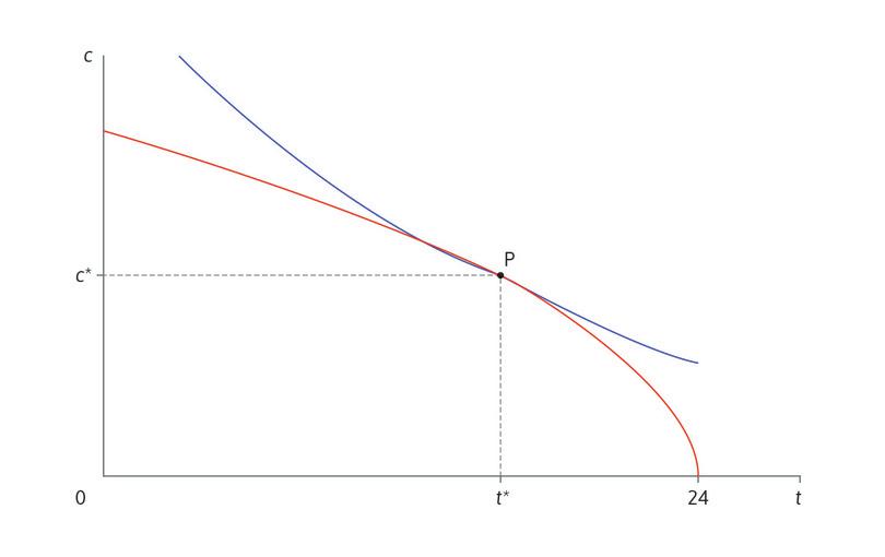
Since $v''(t)$ and $g''(t)$ are both negative, the left-hand side is a decreasing function of $t$. We can deduce that there is only one value of $t$ that satisfies this equation. This is Angela’s optimal choice of free time, which we call $t^*$. Optimal production and consumption are then found from the feasible frontier: $c^* = g(t^*)$. This optimal allocation is shown as point P in Figure 1 below. The blue curve is an indifference curve and the red curve is Angela’s feasible frontier.

An example

We illustrate the analysis above using specific utility and production functions. Suppose that in Angela’s quasi-linear utility function $U(t,\ c) = v(t) + c ,$ the function $v(t)$ is given by:

$$v(t) = 4\sqrt{t}$$

This is a particular case of the example of quasi-linear utility we described in Leibniz 5.4.1: $U(t,\ c)= b t^\alpha+c$, where $b=4$ and $\alpha= 1/2$.

Secondly, assume that Angela’s production function is $y=2\sqrt{2h}$, where $h$ is hours of work. If she has $24$ hours in the day to allocate between work and free time, $h + t =24$, and the equation of her feasible frontier is $y=g(t) ,$ where:

$$g(t) = 2\sqrt{48 -2t}$$

You can verify that this feasible frontier is downward-sloping ($g'(t)\lt0$) and concave ($g''(t)\lt0$).

As above, we can find the marginal rates of transformation and substitution from the derivatives of $g$ and $v$:

$$\text{MRT} = -g'(t) = \frac{2}{\sqrt{48 -2t}}, \quad \text{MRS} = v'(t) = \frac{2}{\sqrt{t}}$$

$\\\\$At the optimal allocation, $\text{MRT} = \text{MRS}$, so $48 -2t = t$. Angela therefore chooses to have $16$ hours of free time per day and work for $8$ hours. From the production function, Angela’s daily consumption of grain is $2\sqrt{2 \times 8} = 8$ bushels.

Read more: Sections 17.1 to 17.3 of Malcolm Pemberton and Nicholas Rau. 2015. Mathematics for economists: An introductory textbook, 4th ed. Manchester: Manchester University Press.