Leibniz

3.1.3 Concave and convex functions

The concept of diminishing marginal product corresponds to the mathematical property of concavity. By looking at the mathematical idea of concave and convex functions, we can gain some further insights into the economic properties of production functions.

concave function

A function of two variables for which the line segment between any two points on the function lies entirely below the curve representing the function (the function is convex when the line segment lies above the function).

We saw in Leibniz 3.1.2 that in the case of the production function $y = Ah^\alpha$, with $A \gt 0$ and $0 \lt \alpha \lt 1$, the marginal product of labour is diminishing. This means that when we move to the right along the graph of the production function, the slope of the curve decreases. A function with this property is said to be concave.

An implication of concavity (and its algebraic definition) is that ‘the function of the average is greater than the average of the function’. To illustrate what this statement means, suppose that for a function $f(h)$, we take any two values $h_0$ and $h_1$. Then:

$$f\left(\frac{h_0+h_1}{2}\right) \gt \frac{f(h_0)+f(h_1)}{2}$$

The left-hand side is the function of the average of the two values, and the right-hand side is the average of the function of the two values. (To see why the inequality holds, try drawing a concave production function, choosing two values on the horizontal axis, and finding the points on the diagram that correspond to the two averages.)

We can give this property a very neat economic interpretation. To understand what it means, consider the following example.

Suppose that Alexei has a production function like the one above, with $A = 20$ and $\alpha = 0.5$; that is:

$$y = 20\sqrt{h}$$

He has just started at university and is considering two different ways of organizing his time. Because he does not yet know anyone, he thinks the first term might be better spent socializing, so that his average daily hours of study for the end-of-semester exam would be $0$. Having established his position on the social scene, he would return to study with full fervour in the second semester and study $9$ hours a day, every day. From his production function, we find that his grades under this regime would be $20\sqrt{0} =0$ for the first semester exam, and $20\sqrt{9} =60$ for the second semester. His average exam result would thus be $\frac{1}{2}\times 0 + \frac{1}{2}\times 60=30$.

Alternatively, he could work on his social life and academic results more steadily, studying $4.5$ hours a day every day in both semesters. Notice that under this strategy, he gives up the same total hours of free time as under the previous approach—the total inputs are the same. What grades can he then expect? He will get $20\sqrt{4.5} = 42.4$ in each semester, which gives him $42.4$ on average.

Comparing these two possible strategies, Alexei realizes that in his case, slow and steady indeed wins the race, because his total output is higher when hours are constant rather than fluctuating. This is the economic implication of concavity.

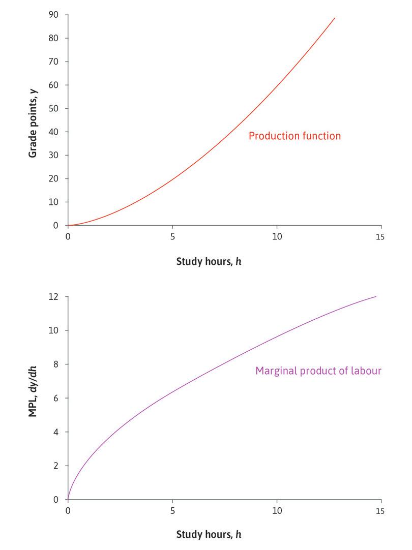
By contrast, had we assumed that $\alpha \gt 1$, we would have found that total output is higher when hours fluctuate: in this case, Alexei learns more when he studies more intensely for a shorter period. When $\alpha \gt 1$, the slope of the graph of the production function increases as hours increase, so the marginal product of labour is increasing rather than diminishing, as in Figure 3 in which $\alpha =1.6$. We would then describe the production function as convex rather than concave. A special case is the function $y=Ah^2$: you can check by differentiating that for this production function, the graph of the marginal product of labour is an upward-sloping straight line.

Read more: Section 8.4 of Malcolm Pemberton and Nicholas Rau. 2015. Mathematics for economists: An introductory textbook, 4th ed. Manchester: Manchester University Press.