Leibniz

5.4.1 Quasi-linear preferences

Angela is a farmer who values two things: grain (which she consumes) and free time. In Unit 5 we assume that her preferences with respect to these two goods have a special property: she values grain at some constant amount relative to free time, independently of how much grain she already has. This Leibniz shows how to capture that property mathematically.

In earlier Leibnizes we have made extensive use of the Cobb-Douglas utility function. We now explore an alternative: the quasi-linear utility function.

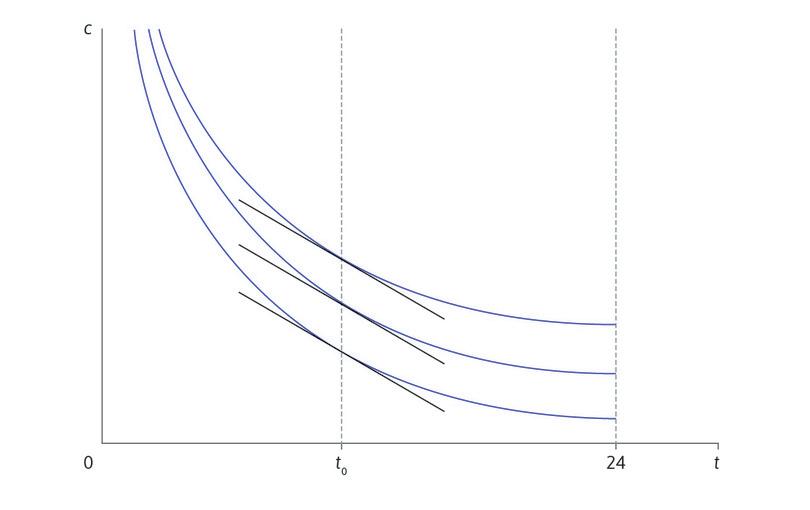
Let $t$ be Angela’s daily hours of free time, and $c$ the number of bushels of grain that she consumes per day. We assume, as in the main text, that the rate at which Angela is willing to exchange grain for free time remains constant as her consumption of grain increases. In other words, her marginal rate of substitution between hours of free time and bushels of grain depends only on the free time and not at all on the grain. We have sketched indifference curves with this property in Figure 1. For any given amount of free time, say $t_0$, the slope of the indifference curve at the point $(t_0,\ c)$ is the same for all $c$, which means that the tangent lines in the figure are parallel.

A utility function with the property that the marginal rate of substitution (MRS) between $t$ and $c$ depends only on $t$ is:

$$U(t,\ c) = v(t) + c$$

where $v$ is an increasing function: $v'(t)\gt0$ because Angela prefers more free time to less. This is called a quasi-linear function because utility is linear in $c$ and some function of $t$. We now show that this utility function has the required property.

Angela’s marginal rate of substitution (MRS) between free time $t$ and consumption of grain $c$ is defined as in Leibniz 3.2.1 as the absolute value of the slope of the indifference curve through the point $(t,\ c)$. It may be found by the formula we derived in the earlier Leibniz:

$$\text{MRS} = \frac{\partial U}{\partial t} \left/ \frac{\partial U}{\partial c} \right.$$

In this case, $\dfrac{\partial U}{\partial t}=v'(t)$ and $\dfrac{\partial U}{\partial c}=1$, so

$$\text{MRS} = v'(t)$$

The same result can be obtained directly, without using the general formula. Each indifference curve is of the form

$$v(t) + c = \text{constant}$$

or $c= k - v(t)$, where $k$ is a constant. Therefore

$$\frac{dc}{dt} = - v'(t) \lt0$$

along an indifference curve. The curve slopes downwards and the absolute value of the slope is $v'(t)$. Thus the MRS is a function of $t$ alone, as we wished to prove.

In Figure 1, the indifference curves have the usual property of diminishing MRS, flattening as you move to the right. For this to happen, $v'(t)$ must fall as $t$ increases. Thus $v''(t)\lt0$: $v$ is a concave function. Because indifference curves are of the form $'c = \text{constant} - v(t)'$, any two of them differ by a constant vertical distance, as you can see in Figure 1. The reason why the curves in the diagram bunch together horizontally at large values of $c$ is simply that they are steeper there.

To summarize: the utility function

$$U(t,\ c) = v(t) + c$$

where the function $v$ is increasing and concave, is called quasi-linear. Using a utility function of this form means that we are making a restrictive assumption about preferences, but it has a very useful implication. Because utility is of the form ‘$c + \text{something}$’, it is measured in the same units as consumption. Angela values $t$ hours of free time as much as $v(t)$ bushels of grain.

The ability to measure utility in consumption units is often helpful, especially in cases where Angela can sell grain on the market and purchase dairy or clothes or anything else with the proceeds. In such contexts, economists often interpret $c$ as money income. The assumption of quasi-linear preferences makes it possible to measure gains and losses of utility in terms of money.

An example

An example of a quasi-linear utility function is:

$$U(t,\ c) = b t^\alpha + c$$

where $b$ and $\alpha$ are positive constants and $\alpha\lt1$. You can see immediately that it has the form $v(t) +c$, with $v(t)= b t^\alpha$. To demonstrate that it is a quasi-linear utility function as described above, we must show that the function $v$ is increasing and concave. This is easily done:

$$v'(t)= \alpha b t^{\alpha -1}$$

which is positive because $b$ and $\alpha$ are positive, and

$$v''(t)= (\alpha -1)\alpha b t^{\alpha -2}$$

which is negative because $b\gt0$ and $0\lt\alpha \lt1$.

Read more: Sections 17.1 to 17.3 of Malcolm Pemberton and Nicholas Rau. 2015. Mathematics for economists: An introductory textbook, 4th ed. Manchester: Manchester University Press.