Leibniz

3.1.1 Average and marginal productivity

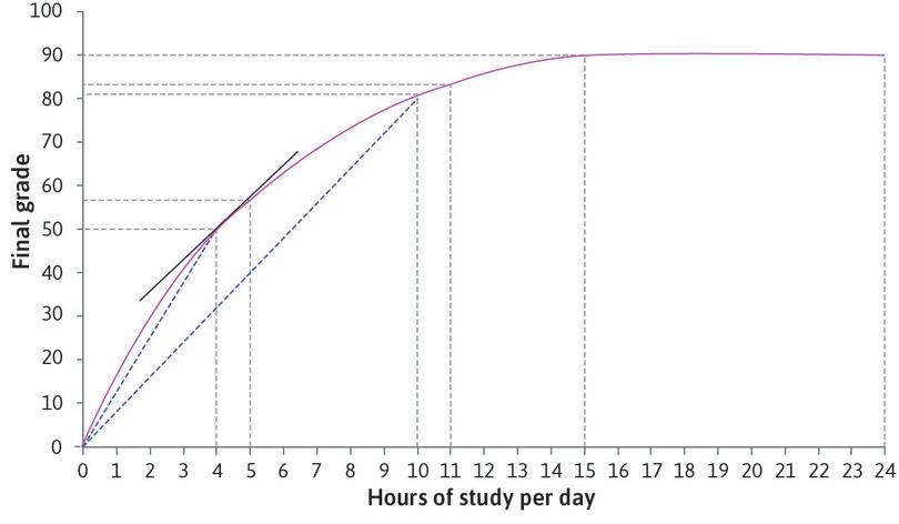
Alexei’s production function, represented graphically in Figure 1, describes how his daily hours of study translate into his final grade. We have seen that his marginal product at each point is the slope of the function, and his average product is the slope of the ray to the origin. Now we look at how to describe the marginal and average products mathematically.

A general mathematical representation of this relationship is:

$$y = f(h)$$

where $y$ is the final grade (his output) and $h$ is hours of study per day (the input). $f(h)$ is the production function.

average product

Total output divided by a particular input, for example per worker (divided by the number of workers) or per worker per hour (total output divided by the total number of hours of labour put in).

When Alexei is studying for $h$ hours per day, his average product of labour (APL) is calculated by dividing the final grade by the number of hours studied:

$$\text{APL} = \frac{y}{h} = \frac{f(h)}{h}$$

This is the average number of grade points per hour of daily study. In the diagram, it is the slope of the ray to the origin.

marginal product

The additional amount of output that is produced if a particular input was increased by one unit, while holding all other inputs constant.

We have defined Alexei’s marginal product of labour (MPL) as the increase in his grade from increasing study time by one hour. More precisely, it is the rate at which his grade increases as study time increases, which corresponds to the slope of the production function.

To see this, suppose that he studies for $h$ hours a day. To find his marginal product, we consider how his grade would change if he increased his study time by $\Delta h$ hours. If the grade increase by $\Delta y$, then the change in grade per unit change of study time is:

$$\frac{\Delta y}{\Delta h} = \frac{f(h + \Delta h) - f(h)}{\Delta h}$$

As $\Delta h$ tends towards zero, this fraction tends towards the derivative of the function. We write:

$$\text{as } \Delta h \to 0, \quad \frac{\Delta y}{\Delta h} \to \frac{dy}{dh}$$

which is the slope of the production function. In other words, Alexei’s marginal product when he studies for $h$ hours is given by the derivative of the production function:

$$\text{MPL} = \frac{dy}{dh}=f'(h)$$

This is the calculus definition of marginal product. We shall be using calculus definitions of marginal quantities in subsequent Leibnizes. In the text we calculated the marginal product by finding the increase in output when the input increases by one unit. This gives a good approximation to the marginal product as defined by calculus if individual units are small quantities. For example, in Figure 1 the units are hours, and there are 24 hours on the horizontal axis. The increase in output when the input rises by one hour is a rough approximation to the slope. But if we put minutes on the horizontal axis instead, and calculated the increase in output when the input rises by a minute, we would obtain a very close approximation to the slope of this function.

An example

A production function with properties similar to that of Figure 1 is:

$$y = Ah^\alpha$$

where $A$ and $\alpha$ are constants such that $A \gt 0$ and $0 \lt \alpha \lt 1$; they determine the precise location and curvature of the production function. We shall explain below why $\alpha$ is restricted to lie between 0 and 1. Notice that this function has the standard properties of a production function: $y=0$ when $h=0$, and when $h$ is positive, output $y$ is also positive.

The restriction $\alpha \gt 0$ ensures that the production function is increasing for all $h \geq 0$ (this may be clear to you from what you know about exponents (powers), but we will verify it below by showing that the marginal product is positive). This means that the function is not an exact representation of the one in Figure 1, which is constant (flat) for $h \gt 15$.

The average product of labour is then:

$$\text{APL} = \frac{y}{h} = \frac{ Ah^\alpha }{h} = Ah^{\alpha-1}$$

The marginal product of labour is the derivative of the production function:

$$\text{MPL} = \frac{dy}{dh} = A\alpha h^{\alpha -1}$$

Note that we can rewrite the MPL as:

$$\text{MPL} = \frac{\alpha}{h} \times Ah^\alpha = \frac{\alpha y}{h}$$

We know that when $h$ is positive, $y$ is positive too. So from this equation you can easily see that $\alpha \gt 0$ implies that the marginal product of labour is positive – in other words, Alexei’s grade increases with hours studied.

How about the restriction $\alpha \lt 1$? Since the average product of labour is $\frac{y}{h}$ and the marginal product of labour is $\frac{\alpha y}{h}$, $\alpha$ is the ratio of the marginal product to the average product. So our assumption that $\alpha \lt 1$ means that the marginal product of labour is less than the average product of labour. You can see this in Figure 1 if you compare the MPL (the slope of the curve) and the APL (the slope of the ray to the origin) shown at the point where $h=4$.

This property of the production function implies that no matter how many hours of study Alexei chooses, the additional grade points he would get for one extra hour of study would be less than the average points per hour that he has earned so far.

Read more: Section 6.1 and Section 6.4 of Malcolm Pemberton and Nicholas Rau. 2015. Mathematics for economists: An introductory textbook, 4th ed. Manchester: Manchester University Press.