Leibniz

8.4.1 The firm and market supply curves

In our model of a city with many small bakeries and many consumers, each bakery is a price-taker in the market for bread. The supply curve of an individual bakery is determined by its marginal cost curve. The market supply at a given price is the total amount of bread that will be supplied by all the bakeries together. This Leibniz explains how to find the firm and market supply curves mathematically.

Suppose there are $m$ bakeries in the city, and the $i^{th}$ bakery has a total cost function $C_i(Q_i)$, where $Q_i$ is the quantity of bread that it produces, for $i = 1,\ …,\ m$. All the bakeries are price-takers. We will first determine the supply functions of the individual bakeries, and then add them together to determine the market supply.

The supply function of bakery $i$

Bakery $i$ takes the market price, $P$, as given, and chooses its quantity $Q_i$ to maximize its profit, which is given by:

$$\Pi_i = PQ_i-C_i(Q_i)$$

Differentiating with respect to $Q_i$ and setting the derivative equal to zero gives us the first-order condition:

$$P = C_i'(Q_i)$$

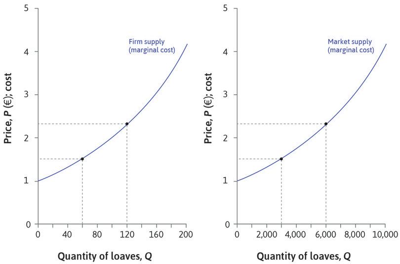
which can be interpreted as saying that the firm will choose its quantity such that the marginal cost is equal to the market price. For each possible value of $P$ there is a corresponding optimal quantity $Q_i$ satisfying this equation. Since the equation tells us the value of $P$ at which the firm would supply quantity $Q_i$, it can be described as the firm’s inverse supply function. Figure 8.7 of the text, reproduced below as Figure 1, shows the firm’s marginal cost, or equivalently its inverse supply function, $P = C_i'(Q_i)$, in the left-hand panel.

The inverse of this function is the direct supply function; it tells us the value $Q_i$ that the firm will choose for a given value of $P$. We will write the firm’s supply function as:

$$Q_i = Q_i^S(P)$$

For example, suppose firm $i$ has cost function $C_i(Q_i) = 3 Q_i^2+2Q_i$. Then by calculating the marginal cost we find that its inverse supply function is $P = 6 Q_i+2$. Rearranging this equation to find $Q_i$ in terms of $P$ gives us the supply function: $Q_i^S(P) = (P-2)/6$.

The market supply function

When the market price is $P,\ Q_1^S (P),\ Q_2^S (P),\ \ldots,\ Q_m^S (P)$ are the individual quantities supplied by the $m$ firms. If the firms all had the same cost functions, they would have identical supply functions; if not, their supply functions will differ. The quantity supplied to the whole market at price $P$ is:

$$Q^S(P) = \sum_{i = 1}^m Q_i^S (P)$$

The function $Q^S(P)$ is the market supply function. The graph of this function, typically drawn with $P$ on the vertical axis and $Q$ on the horizontal, is the market supply curve. Graphically, the process of going from the supply curves of individual firms to that of the whole market can be viewed as aggregation in the horizontal direction; at any particular price, the individual supplies are added up to give the market supply. In Figure 1, we have drawn the market supply in the right-hand panel, on the assumption that there are 50 bakeries ($m = 50$) with identical supply functions. So at each price, market supply $Q^S(P)$ is 50 times the individual firm supply $Q_i^S(P)$.

As we discussed in the text, the market supply curve can be interpreted as the marginal cost curve for the market as a whole. It gives the minimum price at which sellers are willing to supply a given amount of the good. Since each firm chooses a level of output where price equals marginal cost, each firm that produces a positive amount of output must have the same marginal cost. The market supply curve measures the relationship between total output and the common marginal cost of producing this output. The interpretation of the market supply curve as a marginal cost curve is one reason for the standard practice of drawing supply curves with $P$ on the vertical axis.

Read more: Section 7.4 of Malcolm Pemberton and Nicholas Rau. 2015. Mathematics for economists: An introductory textbook, 4th ed. Manchester: Manchester University Press.