Leibniz

7.8.1 The elasticity of demand

The price elasticity of demand measures the sensitivity of quantity demanded to price: it tells us the percentage change in quantity demanded when price changes by 1%. In this Leibniz, we define the elasticity using calculus, and show how the pricing decisions of a firm depend on the elasticity of the demand that it faces.

There are two ways of writing a demand function. Previously we have described the demand for Beautiful Cars using the inverse demand function:

$$P = f(Q)$$

where $f(Q)$ is the price at which the company can sell exactly $Q$ cars. To define the elasticity it is more convenient to write the demand function in its direct form:

$$Q = g(P)$$

$g(P)$ is the quantity of Beautiful Cars demanded if the price is $P$. (The function $g$ is the inverse function of $f$; mathematically, we can write $g(P)=f^{-1}(P)$.)

The derivative of the demand function is $dQ/dP=g'(P)$. This is one way of measuring how much consumer demand $Q$ changes in response to a change in price. But it is not a very useful measure, since it depends on the units in which $P$ and $Q$ are measured. For example, we would get a different answer if the price were in euros, rather than dollars.

Instead, we defined the price elasticity of demand in the text as:

$$-\frac{\%\text{ change in quantity demanded}}{\%\text{ change in price}}$$

This is a more useful measure of the responsiveness of demand to price. You can see from the definition that it is independent of the units of measurement. But it is closely related to the derivative $g'(P)$—to see this, suppose the price changes from $P$ to $P + \Delta P$, causing quantity demanded to change from $Q=g(P)$ to $Q + \Delta Q$. The percentage change in price is $100 \Delta P/P$, and the percentage change in quantity is $100 \Delta Q/Q$. Substituting these in the expression for the elasticity, we obtain:

$$-\frac{ \Delta Q}{Q} \left/ \frac{\Delta P}{P} \right. = -\frac{P}{Q} \, \frac{ \Delta Q}{ \Delta P}$$

Taking the limit of this expression as $\Delta P \to 0$ gives us the calculus definition of the price elasticity of demand, which we denote by $\varepsilon$ as in the text:

$$\varepsilon = - \frac{P}{Q} \, \frac{ dQ}{dP}$$

And since $Q=g(P)$, the elasticity can also be written as:

$$\varepsilon = -\frac{Pg'(P)}{g(P)}$$

Notice that the value of the elasticity is normally positive, since according to the Law of Demand, the derivative of the demand function will be negative.

When defined like this, using calculus, $\varepsilon$ is only approximately the same as our original definition of the elasticity as the percentage fall in quantity demanded when price rises by 1%. But on the reasonable assumption that 1% is a small amount, it is close approximation, and we often interpret it that way.

Consider the demand function:

$$Q=100 P^{-0.8}$$

Here,

$$\varepsilon=-\frac{P}{Q}\,\frac{dQ}{dP} = -\frac{P}{100P^{-0.8}}\times -80P^{-1.8} = 0.8$$

In this particular case, the elasticity of demand is constant—it is equal to $0.8$ at all points on the demand curve.

In general, elasticities are not constant. They vary as we move along the demand curve. But the example above illustrates a special case. If the form of the demand function is $Q = aP^{-c}$, where $a$ and $c$ are positive constants, the elasticity of demand is $c$. This is the only class of demand functions for which the elasticity is constant.

Expressing elasticity in terms of quantity

Another expression for the elasticity of demand may be obtained by returning to the inverse demand function $P=f(Q)$. By the inverse function rule,

$$\frac{dP}{dQ} = 1 \left/ \frac{dQ}{dP} \right.$$

so

$$\varepsilon = - \frac{P}{Q} \left/ \frac{dP}{dQ} \right. = - \frac{f(Q)}{Qf'(Q)}$$

A second example: suppose Beautiful Cars faces the inverse demand function

$$P= 8000 - 80 Q$$

as in Figure 7.15 of the text. Using the expression above, the elasticity of demand is:

$$\varepsilon=-\frac{8,000 -80 Q}{Q\times -80} = \frac{100}{Q} - 1$$

Alternatively, we may express the elasticity in terms of price: $Q=\dfrac{8,000-P}{80}$, so

$$\varepsilon= -\frac{P}{Q}\, \frac{dQ}{dP} = -\frac{80P}{8,000 -P} \times -\frac{1}{80} = \frac{P}{8,000 -P}$$

Each of the two expressions for $\varepsilon$ shows that it falls as we move to the right along the demand curve, increasing $Q$ and reducing $P$. This is so for every linear demand function, as is the result that $\varepsilon$ approaches $0$ as $P$ approaches $0$ and $\varepsilon$ approaches $\infty$ as $P$ approaches its maximum value, where $Q=0$. Thus if Beautiful Cars sells only two cars per day at a price of $7,840, elasticity of demand is 49; while if the company sells 95 cars per day by charging only $400 per car, $\varepsilon=0.053$ to three decimal places.

Elasticity and marginal revenue

We saw in Leibniz 7.6.1 that if Beautiful Cars’ inverse demand function is $f(Q)$, its revenue function is

$$R(Q) = Qf(Q)$$

and that marginal revenue (MR) is defined as follows:

$$\text{MR} = R'(Q) = f(Q) + Qf'(Q)$$

Rewriting this expression using the formula $\varepsilon=-\dfrac{f(Q)}{Qf'(Q)}$ and using the fact that $P=f(Q)$, we see that there is a relationship between marginal revenue and the elasticity of demand:

$$\text{MR} = f(Q) - \frac{f(Q)}{\varepsilon} = P\left(1 - \frac{1}{\varepsilon}\right)$$

This implies that marginal revenue will be positive if $\varepsilon\gt1$, negative if $\varepsilon\lt1$.

As was noted in the text, demand is said to be elastic if $\varepsilon\gt1$, inelastic if $\varepsilon\lt1$. The second example shows that demand may be elastic and inelastic at different points of the same demand curve. What we have just shown is that marginal revenue is positive if, and only if, the firm is operating on that portion of the demand curve where demand is elastic. In particular, this will be so if the firm maximizes its profit and therefore chooses its output to equate marginal revenue and marginal cost, since the marginal cost is positive.

The markup

Recall from Leibniz 7.6.1 that the first-order condition for profit-maximization is $\text{MR} = \text{MC}$, where $\text{MC}$ is marginal cost. Using the formula for marginal revenue that we have just derived, we may write the first-order condition as follows:

$$(\varepsilon -1)P = \varepsilon \, \text{MC}$$

Rearranging,

$$\frac{P - \text{MC}}{P} = \frac{1}{\varepsilon}$$

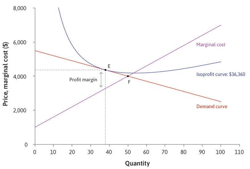
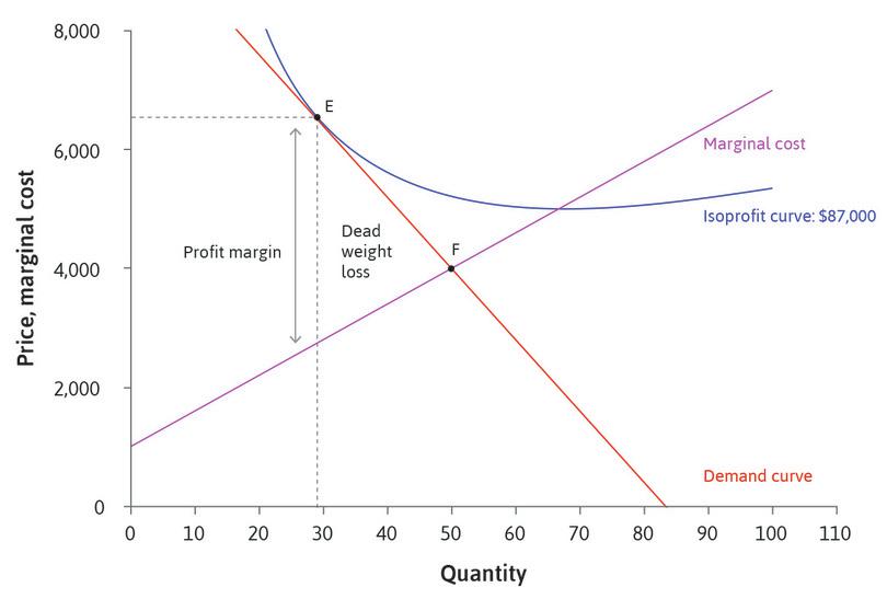
The left-hand side of this equation is the firm’s markup—that is, the profit margin $P-\text{MC}$ as a proportion of the price. The equation tells us that the markup (at the profit-maximizing point) will be greater, the smaller the elasticity of demand. For example, if the elasticity of demand is $5$ at the optimum, there is a markup of $20\%$, whereas an elasticity of demand of $1.25$ means that the markup is $80\%$, so the firm will set its price at five times marginal cost. The inverse relationship between the markup and the price elasticity of demand is illustrated by Figures 7.16 and 7.17 of the text, reproduced below as Figure 1.

Elasticity in general

Elasticity is a general mathematical concept, though as far as we know, only economists use it. Suppose we have a differentiable function $y=F(x)$, where $x$ and $y$ take only positive values. The elasticity of $y$ with respect to $x$ may be defined as:

$$\frac{x}{y} \, \frac{dy}{dx} = \frac{xF'(x)}{F(x)}$$

This is the limit of the ratio

$$\frac{\%\text{ change in } y}{\%\text{ change in } x}$$

as the denominator approaches zero. An alternative, which we used in the case of the price elasticity of demand, is to define the elasticity as the absolute value of this limit.

Read more: Sections 6.4 and 7.4 of Malcolm Pemberton and Nicholas Rau. 2015. Mathematics for economists: An introductory textbook, 4th ed. Manchester: Manchester University Press.