Leibniz

8.6.1 Shifts in demand and supply

The competitive equilibrium price and quantity lie at the point where the supply and demand curves cross. If a shock occurs that shifts one of the curves, the equilibrium price and quantity both change. In this Leibniz, we show how to model the effects of a supply or demand shock mathematically.

To find the competitive equilibrium price and quantity in a market, we need to solve a pair of simultaneous equations—the demand curve $Q=Q^D(P)$, and the supply curve $Q=Q^S(P)$—for P and Q. In competitive equilibrium the price equalizes demand and supply:

$$Q^D(P)=Q^S(P)$$

As we saw in Leibniz 8.4.2, if we know the demand and supply functions we can find the equilibrium price by solving this equation, and hence find the equilibrium quantity. But what happens when one of these functions changes?

Consider the case that we analysed in Leibniz 8.4.2, of a market in which the supply and demand functions are both linear:

$$Q^D(P)=a-bP, \quad Q^S(P)=c+dP$$

where $a, b, c, d$ are constants. Assume as before that a, b and d are all positive, thereby ensuring that the demand curve slopes downward and the supply curve slopes upward; hence there is at most one equilibrium price. Provided that $a \gt c$ and $ac + bd \gt 0$, we showed before that there is a positive equilibrium price $P^*$ and a positive equilibrium quantity $Q^*$, given by:

$$P^*=\frac{a-c}{b+d}, \quad Q^*= a-bP^* = \frac{ad+bc}{b+d}$$

Suppose that in this market there is a positive demand shock. The quantity demanded is now higher at any given price. We can model a demand shock as a change $\Delta a$ in the parameter a. The new demand curve is $Q=a+\Delta a-bP$, where $\Delta a \gt 0$ corresponds to a positive shock—$\Delta a \lt 0$ would imply a negative shock in which the quantity demanded fell at each price.

To find the new equilibrium price and quantity we could solve for $P^*$ and $Q^*$ again, using the new demand curve. But it is quicker and easier to focus on the solutions above for $P^*$ and $Q^*$, and work out how they change when a changes:

$$\Delta P^*=\frac{\Delta a}{b+d}, \quad \Delta Q^*= \frac{d\Delta a}{b+d}$$

If you are not sure where these results come from, you can obtain them by writing down an intermediate step. For example, the change in $P^*$ is given by:

$$\Delta P^*=\frac{a+\Delta a-c}{b+d}-\frac{a-c}{b+d}=\frac{\Delta a}{b+d}$$

It is immediately clear from the expressions for $\Delta P^*$ and $\Delta Q^*$ that an increase in demand ($\Delta a \gt 0$) increases both the equilibrium price and the equilibrium quantity. Notice that if quantity demanded at any price increases by one unit ($\Delta a = 1$) then the increase in quantity demanded and supplied in equilibrium is $d/(b+d)$, which is positive but less than $1$. Thus the increase in demand means that consumers buy more, but it also increases the price, and the consumers buy less than they would have done without the price change.

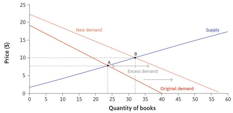
The demand shock we have analysed here is quite similar to the example of an increase in demand for books shown in Figure 8.11 from the text, reproduced as Figure 1 below. The supply and demand functions for books are linear, and the diagram shows that if the number of books increases at each price, the demand curve shifts to the right and the equilibrium price and quantity both rise. The only difference is that a change $\Delta a$ in the parameter a causes a parallel shift of the demand curve, while in Figure 1 the slope also changes.

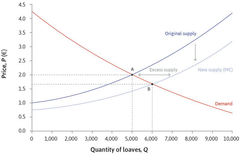
In the text, we also considered an example of a positive supply shock. A technological improvement that allowed bakeries to produce more at a lower price. We depicted this in Figure 8.12, reproduced as Figure 2 below. (The supply and demand curves in this graph are not linear, but the principle is the same.) When the marginal cost of baking falls, the supply curve of bakeries shifts down, and the new market equilibrium is at point B.

Such a supply shock means that bakeries are willing to supply more bread at any given price. It may be represented in our linear example by a change $\Delta c \gt 0$ in the parameter c. (Again, $\Delta c \lt 0$ would mean that firms would supply less bread at each price.) The effect on equilibrium price and quantity of such a change is as follows:

$$\Delta P^*= - \frac{\Delta c}{b+d}, \quad \Delta Q^*= \frac{b\Delta c}{b+d}$$

(As before, write down the intermediate step if you are not sure how to obtain these results.)

In this case we can conclude that, since $\Delta c \gt 0$, the effect of the shock is to increase quantity and reduce price—as can be seen in Figure 2.

The non-linear case

If the demand and supply curves are non-linear, it can be difficult to find an explicit solution for the equilibrium price and quantity. But it is still possible to model the effect of a shock that shifts one of the curves, and work out how it affects the equilibrium. We did this diagrammatically in the text for the bread market example. Here we do the same thing algebraically.

We will write the demand curve for bread as $Q=Q^D(P,\ a)$. The quantity demanded decreases with the price P, as before; but it also depends on a parameter a, which captures consumer tastes. A high value of a represents a situation in which consumers have a strong liking for bread, so will purchase a high quantity at any given price. When a is low, less bread is demanded at each price. The dependence of demand on P and a can be described using the partial derivatives:

$$\frac{\partial Q^D}{\partial P} \lt 0; \quad \frac{\partial Q^D}{\partial a} \gt 0$$

Then a positive demand shock can be represented as an increase in the parameter a. It has the effect of increasing the quantity demanded at each price. When the demand curve is drawn in $(Q,\ P)$ space, as usual, it is drawn for a fixed value of a. An increase in a shifts the demand curve to the right. Similarly, a fall in a represents a negative demand shock and shifts the curve to the left.

In the same way, we will write the supply curve for bread as $Q=Q^S(P,\ c),$ where the parameter c is introduced to model supply shocks. We can think of c as representing technology. A rise in c corresponds to a technological improvement, which lowers the marginal cost of producing bread and hence implies that bakeries will supply more bread at any given price. In terms of partial derivatives:

$$\frac{\partial Q^S}{\partial P} \gt 0; \quad \frac{\partial Q^S}{\partial c} \gt 0$$

An improvement in technology is modelled as an increase in c, shifting the supply curve to the right. This is the case illustrated in Figure 2.

For any given a and c, the demand curve is downward-sloping and the supply curve is upward sloping in $(Q,\ P)$ space. Hence there is at most one equilibrium price $P^*,$ and corresponding equilibrium quantity $Q^*.$ But if a and c change, $P^*$ and $Q^*$ will change too. So $P^*$ and $Q^*$ depend on a and c, and we can express this by writing them as functions:

$$P^* = F(a,\ c), \quad Q^* = G(a,\ c)$$

We want to know how $P^*$ and $Q^*$ change when a and c change. In other words, we want to know the signs of the partial derivatives of $P^*$ and $Q^*$ with respect to a and c. To find them, we use the technique of implicit differentiation. We will start with the partial derivatives with respect to a. These will tell us the effect of a demand shock on the equilibrium.

The equilibrium price $P^*$ satisfies the market-clearing equation:

$$Q^D(P^*,\ a)=Q^S(P^*,\ c)$$

We will differentiate both sides of this equation with respect to a, remembering that $P^*$ is a function of a (that is, $P^* = F(a,\ c)$). We obtain:

$$\frac{\partial Q^D}{\partial P} \frac{\partial P^*}{\partial a}+ \frac{\partial Q^D}{\partial a} =\frac{\partial Q^S}{\partial P} \frac{\partial P^*}{\partial a}$$

This equation can be rearranged, to write $\partial P^*/\partial a$ in terms of the other partial derivatives:

$$\frac{\partial P^*}{\partial a} =\frac{\frac{\partial Q^D}{\partial a}} {\frac{\partial Q^S}{\partial P}-\frac {\partial Q^D}{\partial P} }.$$

The denominator of this fraction is positive, because we know that $\partial Q^S/\partial P \gt 0$ and $\partial Q^D/\partial P \lt 0$. The numerator is positive too, from the way we specified the demand function, above. Hence we can conclude that $\partial P^*/\partial a \gt 0$. Thus, a positive demand shock (an increase in a) leads to an increase in the equilibrium price.

To find $\partial Q^*/\partial a$, we can use the equation for $Q^*$:

$$Q^*=Q^S(P^*,\ c)$$

again remembering that $P^*$ is a function of a. Differentiating with respect to a:

$$\frac{\partial Q^*}{\partial a} =\frac{\partial Q^S}{\partial P^*} \frac{\partial P^*}{\partial a}$$

From this expression, since $\partial Q^S/\partial P^*\gt0$ and we have just shown that $\partial P^*/\partial a\gt0$, we deduce that $\partial Q^*/\partial a\gt0$ too. Thus, a positive demand shock (an increase in a) leads to an increase in both the equilibrium price and the equilibrium quantity, and a negative demand shock has the opposite effects.

To find the effect of a supply shock, we need to find the partial derivatives of $P^*$ and $Q^*$ with respect to c. This can be done in just the same way. We start by differentiating the market-clearing equation with respect to c, to obtain an expression for $\partial P^*/\partial c$ that we can sign. Then we use either the equation for the supply curve or the equation for the demand curve (the latter is easier in this case) to sign $\partial P^*/\partial c$. If you do this carefully, you should find that $\partial P^*/\partial c\lt0$ and $\partial Q^*/\partial c\gt0$, so a positive supply shock raises quantity and lowers price.

This analysis has demonstrated that the qualitative effects of demand and supply shocks on the equilibrium price and quantity are the same as the ones we saw diagrammatically in the text, whatever the precise form of the supply and demand functions—provided that they have the standard properties. That is, the demand curve slopes downward, and the supply curve slopes upward.

Read more: Section 15.2 and the first two paragraphs of Section 15.3 of , Malcolm Pemberton and Nicholas Rau. 2015. Mathematics for economists: An introductory textbook, 4th ed. Manchester: Manchester University Press.