Unit 14 Unemployment and fiscal policy
Themes and capstone units
How governments can moderate costly fluctuations in employment and income
- Fluctuations in aggregate demand affect GDP growth through a multiplier process, because households face limits to their ability to save, borrow, and share risks.
- An increase in the size of government following the Second World War coincided with smaller economic fluctuations.
- Governments can use changes in taxes or government spending to stabilize the economy, but bad policy can destabilize it.
- If a single household saves, its wealth necessarily increases, but if all households save this may not be true, because without additional spending by the government or firms to counteract the fall in demand, aggregate income will fall.
- Every national economy is embedded in the world economy. This is a source of shocks, both good and bad, and places constraints on the kinds of policies that can be effective.
In August 1960, three months before he was elected US president, the 43-year-old Senator John F. Kennedy found time to spend the day cruising Nantucket Sound on his boat, the Marlin. His crew for the day included John Kenneth Galbraith and Seymour Harris, both Harvard economists, and Paul Samuelson, an economist at MIT and later also a Nobel laureate. They had not been recruited for their nautical skills. In fact, apart from Harris, the senator did not even know them.
The future president wanted to learn ‘the new economics’, which John Maynard Keynes, an economist who we will learn more about in Section 14.6, had formulated in response to the Great Depression. When Kennedy was a teenager in the decade before the Second World War, the US and many other countries experienced a drastic fall in output (we can see this for the US in Figure 14.1) and massive unemployment that persisted for more than 10 years.
Kennedy had a lot to learn. He admitted that he had barely passed the only economics course he took at Harvard. He would later spend a day at the America’s Cup sailing races being tutored by Harris, who assigned texts for him to read. Harris later gave private lessons to the senator, shuttling by air between Boston, where he worked, and Washington DC.
In 1948, Samuelson had written Economics, the first major textbook to teach these new ideas. Harris promoted the same economic ideas in a book that he edited in 1948 called Saving American Capitalism, a collection of 31 essays by 24 contributors. At that time, it seemed that capitalism needed saving: the centrally planned economies of the Soviet Union and its allies, a model promoted as the alternative to capitalism, had entirely avoided the Great Depression. Kennedy needed economics to understand policies that could promote economic growth, reduce unemployment, but also avoid economic instability.
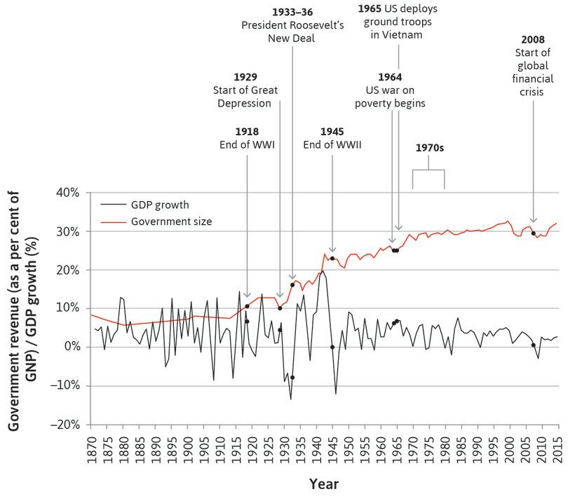
We have seen in Unit 13 that instability in the economy as a whole is characteristic not only of economies dominated by agriculture, but also of capitalist economies. Figure 14.1 shows the annual growth of real GDP in the US economy since 1870.
Fluctuations in output and the size of government in the US (1870–2015).
Figure 14.1 Fluctuations in output and the size of government in the US (1870–2015).
The Maddison Project. 2013. 2013 Version; US Bureau of Economic Analysis. 2016. GDP & Personal Income; World Bank; Wallis, John Joseph. 2000. ‘American Government Finance in the Long Run: 1790 to 1990’. Journal of Economic Perspectives 14 (1) (February): pp. 61–82.
A dramatic reduction in the severity of business cycles occurred after the end of the Second World War. Figure 14.1 shows another important development at that time: the increasing role of the government in the economy. The red line shows the share of federal (national), local, and state government tax revenue as a share of GDP. This is a good measure of the size of the government relative to that of the economy.
The share of employment in agriculture, which we have seen was one cause of volatility in the economy, fell from 50% in the 1870s to 20% by the beginning of the Second World War, yet there was no sign of the economy becoming more stable over this period. As we have seen, households try to smooth fluctuations in their consumption but they can’t always do this successfully, partially because there are limits to how much they can borrow.
The fact that the fluctuations in output growth dramatically reduced while the size of government expanded does not mean that increased government spending stabilized the economy (remember: statistical correlations do not mean causation). But there are good reasons to think that the increase in the red line was part of the reason for the smoothing of the black line. In this unit, we ask why the increased role of the government in the economy is part of the explanation for the more stable economy in the second half of the twentieth century.
What Harris taught Kennedy was influenced by the contrast between the volatility of the economy before the Second World War, and the steadier growth and absence of deep recessions afterwards. Why do economies experience unemployment, inflation, and instability in output, and what kinds of policies might address these problems?
- great moderation
- Period of low volatility in aggregate output in advanced economies between the 1980s and the 2008 financial crisis. The name was suggested by James Stock and Mark Watson, the economists, and popularized by Ben Bernanke, then chairman of the Federal Reserve.
In Unit 13, we took the household‘s viewpoint of the business cycle, which allowed us to establish why fluctuations in employment and income are costly, and how households try to limit the consequences for their wellbeing. In this unit, we take the policymaker’s viewpoint. As we saw in Figure 14.1, the big increase in the size of government after the Second World War was accompanied by a reduction in the size of business cycle fluctuations. After 1990, the business cycle in advanced economies became even smoother, until the global financial crisis in 2008. This led to the period from the early 1990s to the late 2000s being called the great moderation.
14.1 The transmission of shocks: The multiplier process
In a capitalist economy, private investment spending is driven by expectations about future post-tax profits. As we saw in Unit 13, spending on investment projects tends to occur in clusters. Two reasons for this observation are:
- Firms may adopt a new technology at the same time.
- Firms may have similar beliefs about expected future demand.
We need a tool to help us understand how decisions of firms (and households) to raise or reduce investment spending will affect the economy as a whole. You will recall that some households are able to completely smooth temporary bumps in their income, but that in credit-constrained households, higher income from getting a job or moving from part-time to full-time work will also lead to higher consumption spending.
- aggregate demand
- The total of the components of spending in the economy, added to get GDP: Y = C + I + G + X – M. It is the total amount of demand for (or expenditure on) goods and services produced in the economy. See also: consumption, investment, government spending, exports, imports.
As a result, changes in current income influence spending, affecting the income of others, so indirect effects through the economy amplify the direct effect of a shock to aggregate demand (often shortened to AD) created by an investment boom.
We will show how economists answer such questions as ‘how large would the total direct and indirect impact of a rise in investment spending be?’ or, ‘what would be the effect of lower government spending?’
A statistic called the multiplier provides one way of answering this question. Imagine there is a new technology. New spending takes place in the economy as a result; output of the new capital goods rises, as do the incomes of the people producing them. The circular flow of expenditure, income, and output previously shown in Figure 13.6 illustrates this process.
- If the total increase in GDP is equal to the initial increase in spending: We say that the multiplier is equal to 1.
- If the total increase in GDP is greater or less than the initial increase in spending: We say that the multiplier is greater than 1 or less than 1.
- multiplier process
- A mechanism through which the direct and indirect effect of a change in autonomous spending affects aggregate output. See also: fiscal multiplier, multiplier model.
- consumption function (aggregate)
- An equation that shows how consumption spending in the economy as a whole depends on other variables. For example, in the multiplier model, the other variables are current disposable income and autonomous consumption. See also: disposable income, autonomous consumption.
To see why GDP may rise by more than the initial increase in investment spending, we explain what economists call the multiplier process. We do this by combining the very different behaviour of consumption-smoothing and non-smoothing households to represent consumption spending for the economy as a whole. In this aggregate consumption function, consumption depends on current income, among other things. Recall that in the model of Unit 13, consumption-smoothing households will not increase their consumption one-for-one, or even at all, in response to a temporary €1 increase in their income. Credit-constrained and other households who do not smooth, on the other hand, will increase their current consumption by €1 in response to a temporary €1 increase in their income.
In 2008, when governments considered temporary increases in government spending and tax cuts in response to the recession that followed the global financial crisis, the size of the multiplier became the subject of a debate among policymakers and economists. We return to this debate later in the unit.
As we shall see, the multiplier is greater than 1 if the additional consumption spending resulting from a temporary €1 increase in income is greater than zero but less than €1 (say, for example, 60 cents).
After explaining how this is a consequence of the multiplier process, we will show that the validity of the assumptions we make in the multiplier model depend on the state of the economy.
14.2 The multiplier model
- consumption (C)
- Expenditure on consumer goods including both short-lived goods and services and long-lived goods, which are called consumer durables.
- investment (I)
- Expenditure on newly produced capital goods (machinery and equipment) and buildings, including new housing.
We begin with a simple model that excludes the government and foreign trade. In this model, there are two types of expenditure:
- consumption
- investment
We assume that aggregate consumption spending has two parts:
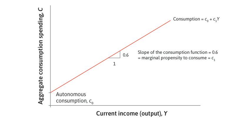
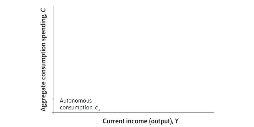
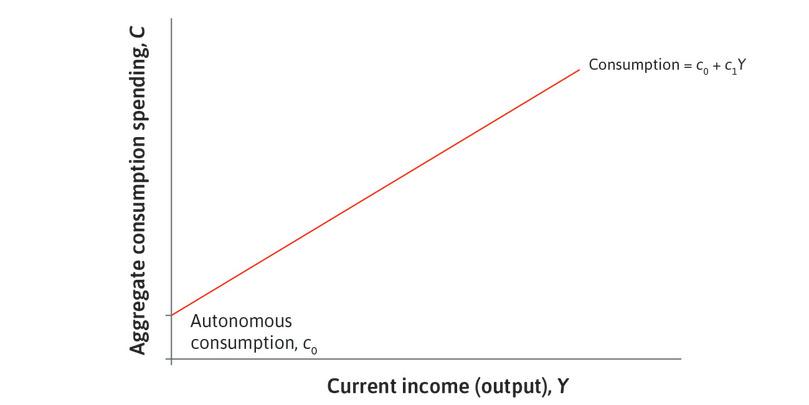
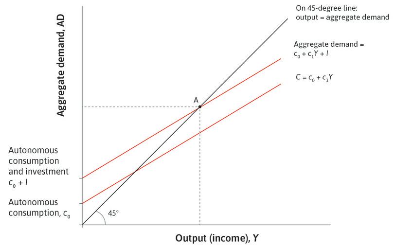
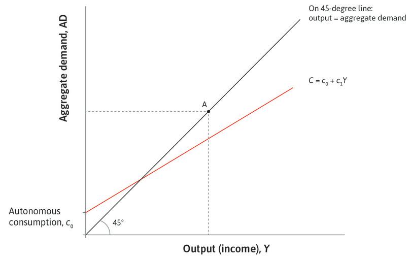
- A fixed amount: How much people will spend, independent of their income. This fixed amount, also known as autonomous consumption, is shown as c₀ on the vertical axis of Figure 14.2.
- A variable amount: This depends on current income, and is an upward-sloping red line in Figure 14.2.
- autonomous consumption
- Consumption that is independent of current income.
So we can write consumption spending in the form of an equation, which we call the aggregate consumption function:
- marginal propensity to consume (MPC)
- The change in consumption when disposable income changes by one unit.
The term c1 gives the effect of one additional unit of income on consumption, called the marginal propensity to consume (MPC). In Figure 14.2, the slope of the consumption line is equal to the marginal propensity to consume. A steeper consumption line means a larger consumption response to a change in income. A flatter line means that households are smoothing their consumption so that it does not vary much when their incomes change. We assume that the marginal propensity to consume is positive, but less than one. This means that only part of an increase in income is consumed; the rest is saved.
We will work with an aggregate consumption function in which the marginal propensity to consume, c1, equals 0.6. This means that an additional unit of income (Euros in this case) increases consumption by €1 × 0.6 = 60 cents.
Naturally, this average number hides large variation across households, who differ in their wealth and in the credit constraints they face. Most households have little wealth, and even in rich countries about one in four households are credit-constrained. As we saw in Unit 13, weakness of will also plays a role. So, both for households that are credit-constrained and for those that do not save ahead of anticipated declines in income, consumption closely tracks income.
Households with low wealth smooth consumption very little if their income falls sharply. The marginal propensity to consume for this group is closer to 0.8. For the small fraction of households who hold the majority of wealth, however, current income plays a very small role in determining consumption, and their marginal propensity to consume is closer to zero. This means that for rich households, an increase in current income of €1 would raise their consumption by just a few cents.
The term c₀ in the aggregate consumption function captures all the other influences on consumption that are not related to current income. Taken literally, it is how much a person with no income would consume, but this is not the best way to think about it. It is just the consumption that is independent of income, and for this reason we call it autonomous consumption.
Since the consumption function only explicitly includes current income, expectations about future income will be included in autonomous consumption. To see what this means in practice, recall from Unit 13 that consumption will change as a result of people becoming more or less optimistic about their future employment and earnings prospects.
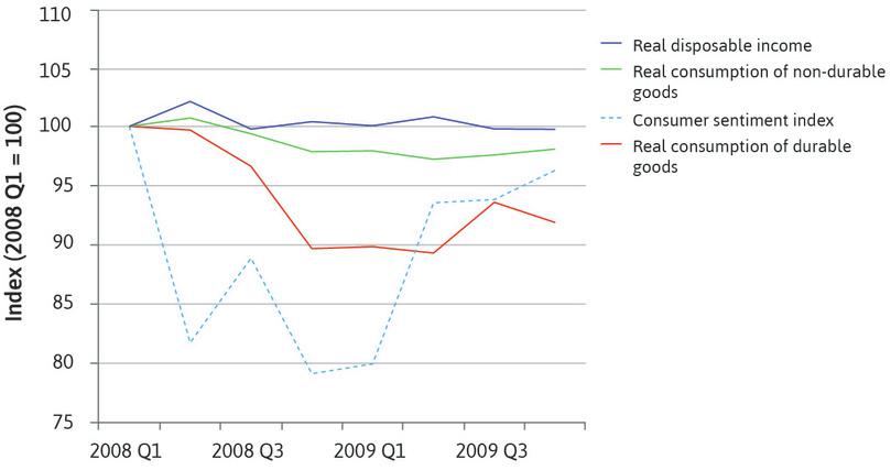
Figure 14.3 illustrates how expectations affected consumption in the financial crisis of 2008 and highlights the exceptional nature of this episode. The figure shows how consumer confidence changed in the US over the course of the crisis. The consumer sentiment index that we have used is the University of Michigan Surveys of Consumers. It is based on monthly interviews with 500 households, and asks how they view prospects for their own financial situation and for the general economy over the short and long term. The figure also plots the evolution of a number of key macroeconomic indicators: disposable income, consumption of durable goods like cars and home furnishings, and consumption of non-durable goods, such as food. All of the series in Figure 14.3 are shown as index numbers, with the first quarter of 2008 as the base year.
Fear and household consumption in the US during the global financial crisis (2008 Q1–2009 Q4).
Figure 14.3 Fear and household consumption in the US during the global financial crisis (2008 Q1–2009 Q4).
Federal Reserve Bank of St. Louis. 2015. FRED.
We notice:
- Consumption of non-durable goods went down slightly more than disposable income: It fell by 3% during the period. Contrary to the predictions of consumption smoothing, households were sufficiently worried about their future prospects that they made adjustments to their spending on non-durables.
- Consumption of durables decreased much more dramatically than disposable income: It decreased by 10% in the first year.
Why the sudden drop in consumption of consumer durables? An important reason is that households were suddenly fearful about the future of their jobs, as shown by the sharp decline in the consumer sentiment index in Figure 14.3. The collapse of the investment bank Lehman Brothers in September 2008, worries about the stability of the banking system, and a higher burden of household debt due to falling house prices led households with mortgages to postpone purchases of expensive items like cars and fridges. It’s important to remember that spending on consumer durables can easily be postponed. In this sense it is more like an investment than a consumption decision (even though consumer durables are counted as part of consumption in the national accounts). As a result, we would expect the series for consumer durables to be more volatile than for non-durable consumption.
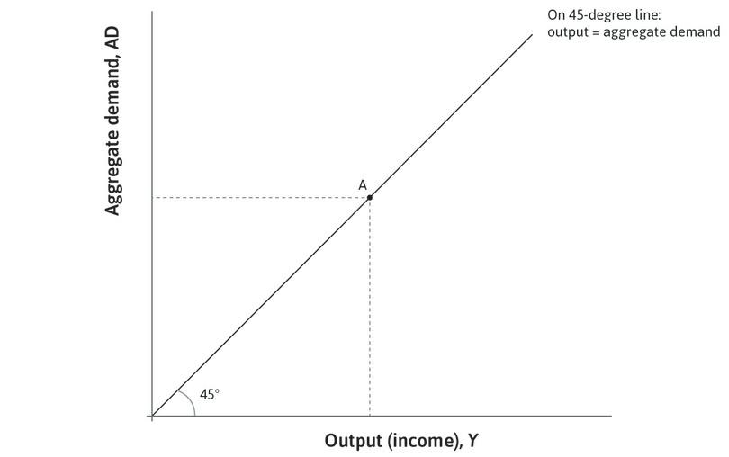
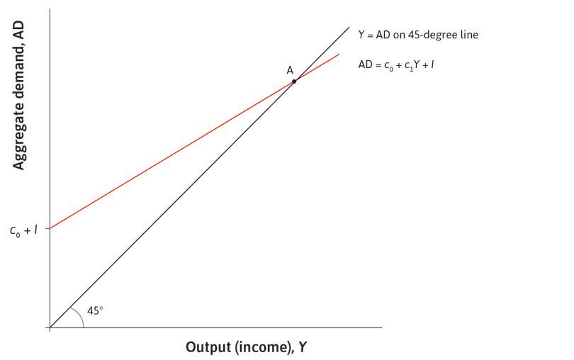
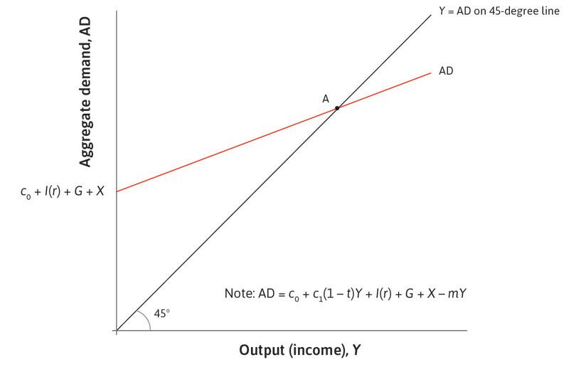
We now show how a shock is transmitted through the economy. In Figure 14.4 we show the amount of output produced by the economy (on the horizontal axis) and the demand for output (on the vertical axis). Everything is measured in real terms because we are interested in how changes in aggregate demand create changes in output and employment.
The 45-degree line from the origin of the diagram shows all the combinations in which output is equal to aggregate demand. This corresponds to the circular flow discussed in Unit 13, where we saw that spending on goods and services in the economy (aggregate demand) is equal to production of goods and services in the economy (aggregate output). You can see this because with a 45-degree line the horizontal distance (output) is equal to the vertical distance (aggregate demand). We can therefore say that:
- goods market equilibrium
- The point at which output equals the aggregate demand for goods produced in the home economy. The economy will continue producing at this output level unless something changes spending behaviour. See also: aggregate demand.
- capacity utilization rate
- A measure of the extent to which a firm, industry, or entire economy is producing as much as the stock of its capital goods and current knowledge would allow.
But how do we know where the economy is on the 45-degree line? Is it at a position of low output, which would mean high unemployment, or is it at a position of high output, which would mean low unemployment?
We determine this position by analysing the individual components of aggregate demand. We assume that firms are willing to supply any amount of the goods demanded by those making purchases in the economy; they are not operating at full capacity utilization. Because we have assumed that there is no government spending or trade with other economies, in this model there are just two components of aggregate spending:
- Consumption: We take the consumption line introduced in Figure 14.2. Because the marginal propensity to consume is less than one, the consumption line is flatter than the 45-degree line, which has a slope of one.
- Investment: We assume investment does not depend on the level of output.
The equation for aggregate demand is therefore:
So adding investment to the consumption line simply leads to a parallel upward shift. In this respect, investment is similar to autonomous consumption. We can see from Figure 14.4 that the aggregate demand line has an intercept of c₀ + I, a slope of c1, and is flatter than the 45-degree line.
In Figure 14.4 we now have a picture showing how the level of output in the economy is determined. Output is equal to aggregate demand (the 45-degree line), and aggregate demand is equal to c₀ + c1Y + I (the flatter line), so the economy must be at point A where the two lines cross.
The same figure tells us the effect of a change in autonomous consumption (c₀) or investment. We study this change exactly as we did the changes in supply and demand in Unit 11: we see how the change makes the old outcome no longer an equilibrium, and then we locate the new equilibrium. The expected change is the movement from the old to the new equilibrium.
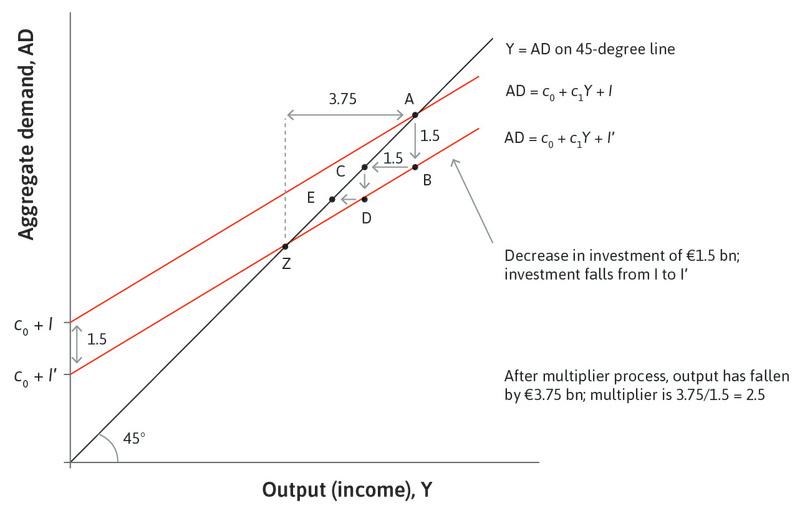
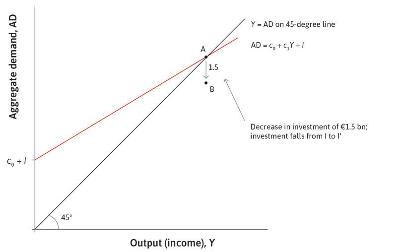
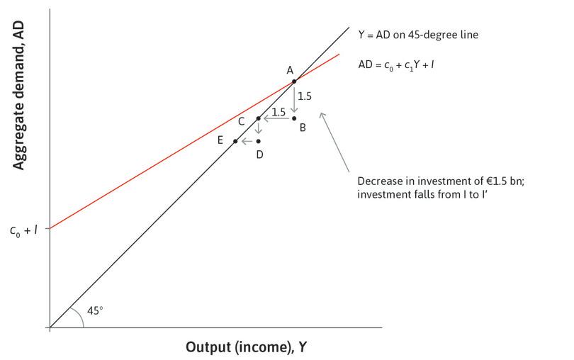
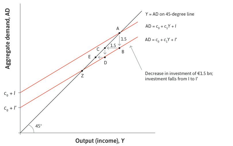
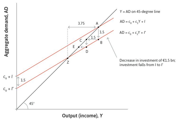
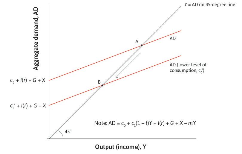
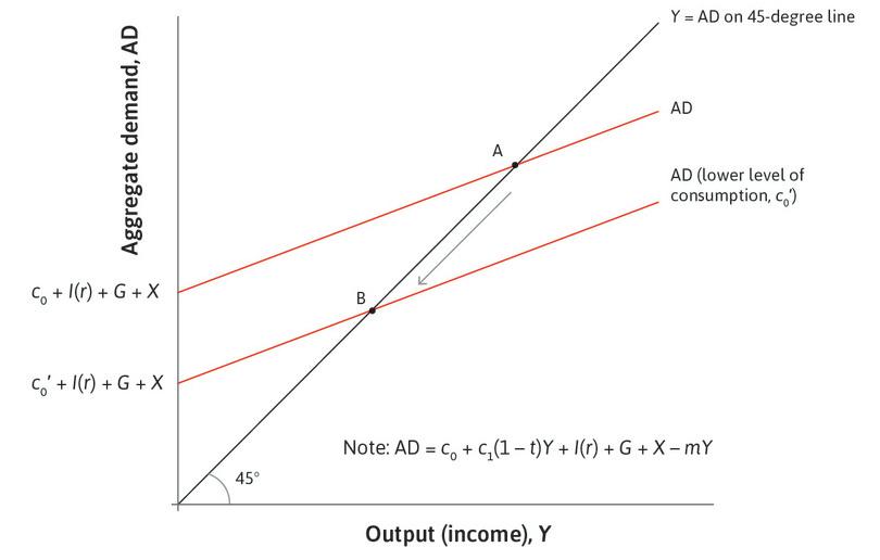
Changes in autonomous consumption or investment displace the old equilibrium because they change aggregate demand, which in turn alters the level of output and employment. In Figure 14.5, we take the multiplier diagram and reduce investment. We choose a reduction in investment of €1.5 billion. Follow the steps in Figure 14.5 to see what happens.
We trace the effect of the fall in investment through the economy in Figure 14.5. The first-round effect is that the fall in investment cuts aggregate demand by €1.5 billion. But lower spending also means lower production and lower incomes, and firms will fire workers as a result, leading to a further decline in spending. Think of credit-constrained households where some members lose their job: they would like to keep consumption stable, but when their income falls they are unable to borrow enough to sustain that level of consumption, so they reduce their spending, which leads to further cuts in production and incomes. The consumption equation tells us that this kind of behaviour leads to a fall in aggregate consumption of 0.6 times the fall in income. The process will go on until the economy reaches point Z.
Following the investment shock, the intercept of the line has moved down by €1.5 billion, causing a parallel shift in the aggregate demand line. Output has fallen by €3.75 billion, more than the fall in investment of €1.5 billion: this is the multiplier process.
In this case, the multiplier is equal to 2.5, because the total change in output is 2.5 times larger than the initial change in investment. A multiplier of 2.5 is unrealistically large. As we shall see in the next section, once taxes and imports are introduced in the model, the multiplier shrinks.
- multiplier model
- A model of aggregate demand that includes the multiplier process. See also: fiscal multiplier, multiplier process.
We call the model of aggregate demand that includes the multiplier process the multiplier model. This is a summary:
- A fall in demand leads to a fall in production and an equivalent fall in income: This leads to a further (smaller) fall in demand, which leads to a further fall in production, and so on.
- The multiplier is the sum of all these successive decreases in production: Eventually, output has fallen by a larger amount than the initial shift in demand. Output is a multiple of the initial shift.
- Production adjusts to demand: Firms supply the amount of goods demanded at the prevailing price. When demand falls, firms adjust production down. The model assumes that they do not adjust their prices.
Note that the economy we are studying is one in which we assume there are underutilized resources in the form of spare capacity in production facilities and underemployed labour. We also assume that wages are not affected by changes in the level of output. For the multiplier process to work in the same way in response to a rise in investment, the assumption of spare capacity and fixed wages means that costs will not rise when output goes up, so firms will be happy to supply the extra output demanded without adjusting their prices. Otherwise some of the increased spending will translate into higher prices or wages rather than higher real output—as we discuss in the next unit.
If the economy is not characterized by spare capacity and constant wages, the multiplier will be smaller than what we find here.
We can also show the effect on output by combining the two equations that determine the lines in the multiplier diagram. The 45-degree line is simply the equation Y = AD. Combining this with the equation for AD gives us:
Collecting terms on the left hand side,
We then divide through by (1 − c1):
- autonomous demand
- Components of aggregate demand that are independent of current income.
We can now calculate how much output will increase or decrease using the value of the multiplier times the change in autonomous demand.
Discover another way to summarize our findings from the diagram algebraically in the Einstein at the end of this section.
The change in output in Figure 14.5 is 2.5 times greater than the initial shock to investment, which means that the shock has been amplified. In algebra, we write this as ΔY = kΔI, and say it as ‘delta Y (the change in output) is equal to k, the multiplier, times delta I (the change in investment)’.
Question 14.1 Choose the correct answer(s)
Figure 14.2 depicts a consumption function of an economy, where C is the aggregate consumption spending and Y is the current income of the economy.
Based on this information, which of the following statements is correct?
- The MPC is the proportion of the additional income received that is spent on consumption. Here it is given by c1. C/Y is the average propensity to consume.
- The slope of the line gives the MPC.
- Households that smooth consumption will increase spending by less than the amount their income increases.
- C is c0 + c1Y, that is, $60 trillion plus the fixed (or autonomous) consumption c0.
Question 14.2 Choose the correct answer(s)
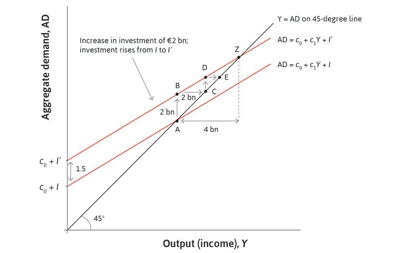
The following diagram depicts the change in the aggregate goods market equilibrium when there is a €2 billion increase in investment.
The economy’s marginal propensity to consume is 0.5. Based on this information, which of the following statements is correct?
- The equilibrium is where the aggregate consumption line intersects with the 45-degree line. Therefore the new equilibrium is Z.
- The diagram shows that the increase in investment results in a €4 billion increase in aggregate demand.
- The multiplier is equal to 1/(1 − 0.5) = 2.
- The distance between A and B is the initial increase in investment of €2 billion. At C, the output Y has increased by €2 billion compared with B, which results in an increase in the aggregate demand of ΔY (change in Y) × MPC, that is, €2 billion × 0.1 = €1 billion.
Einstein Calculating the multiplier
We consider the effect of an increase in investment of €1.5 billion. We can summarize our findings from the multiplier diagram by doing some algebra. To get the multiplier, we can calculate the total increase in production after n + 1 rounds of the process. Each round of the process matches the circular flow diagram. The first-round increase in demand and production is €1.5 billion. The second-round increase in demand and production is (c1 × €1.5 billion), the third-round increase in demand and production is c1 × (c1 × €1.5 billion) = (c12 × €1.5 billion), and so on.
Following this logic, the total increase in demand and production after n + 1 rounds is the total sum of these changes:
Because the marginal propensity to consume is lower than one, we can show that the total sum in the brackets reaches a limit of 1/(1 − c1) as n gets large. This is because the term in the brackets is, mathematically, a geometric series. We show this as follows.
If k is the multiplier, we have:
Now multiply both sides by (1 – c1) to get:
Now divide again by (1 − c1):
As n gets large, assuming c1 < 1, the numerator tends to 1. So, in the limit:
In the example, the marginal propensity to consume is, on average, 0.6. This implies that the multiplier is equal to:
We can then apply the multiplier to the initial change in investment of €1.5 billion to find the sum of all the successive increases in production triggered by the initial hike in investment and aggregate demand: 2.5 × €1.5 billion = €3.75 billion.
14.3 Household target wealth, collateral, and consumption spending
From Unit 13, we know that consumption is the largest component of GDP in most economies. Therefore an important part of understanding changes in output and employment is understanding why consumption changes.
We saw that a shock to investment shifts the aggregate demand curve, and is transmitted through the economy as households adjust their spending in response to changes in income. We focused on incomplete consumption smoothing, such as credit constraints. This behaviour is reflected in the size of the multiplier and the slope of the aggregate demand curve. But consumption and saving behaviour can also shift the aggregate demand curve.
A shift in aggregate demand can be caused by a shift in autonomous consumption, represented by the term c₀ in the aggregate consumption function, C = c₀ + c1Y. A change in c₀ will in turn produce a multiplier response of output and employment through the circular flow of expenditure, output, and income in the same way as the fall in investment in the previous section was multiplied.
- mortgage (or mortgage loan)
- A loan contracted by households and businesses to purchase a property without paying the total value at one time. Over a period of many years, the borrower repays the loan, plus interest. The debt is secured by the property itself, referred to as collateral. See also: collateral.
- precautionary saving
- An increase in saving to restore wealth to its target level. See also: target wealth.
- target wealth
- The level of wealth that a household aims to hold, based on its economic goals (or preferences) and expectations. We assume that households try to maintain this level of wealth in the face of changes in their economic situation, as long as it is possible to do so.
Think about a family with a mortgage on its house. If the price of houses falls, the family will be concerned that its wealth, too, has fallen. A likely reaction to this is for the household to save more. This is called precautionary saving. One way to analyse this behaviour is to assume that households have in mind a target wealth that they aim to hold.
When something happens to affect the stock of the household’s wealth relative to this target, it reacts by either increasing or decreasing its savings to restore wealth back to its target level. If this adjustment involves precautionary saving, it is modelled as a fall in autonomous consumption.
- Great Depression
- The period of a sharp fall in output and employment in many countries in the 1930s.
In 1929, a downturn in the US business cycle that initially appeared similar to others in the preceding decade turned into a large-scale economic disaster—the Great Depression.1
The fall in output and employment during the Great Depression highlights two ways in which aggregate consumption might fall—credit constraints in the multiplier process, and changes in wealth relative to target wealth.
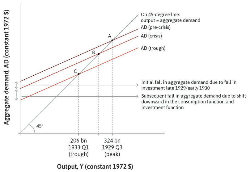
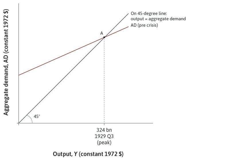
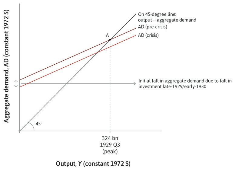
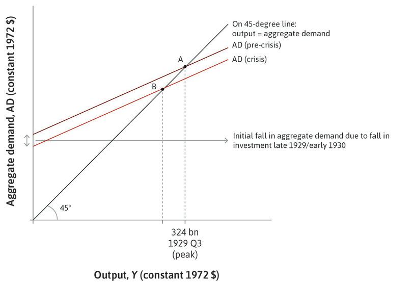
To understand the economic mechanisms at work in the Great Depression, we use the multiplier diagram shown in Figure 14.6. Point A shows the initial situation of the economy in the third quarter of 1929. There was then a fall in investment. This shifts the aggregate demand curve from the pre-crisis to the crisis level. The dotted line from point B shows the level of output that would have been observed in the business cycle trough if the usual multiplier process had been at work. There would have been a recession, but no Great Depression. But the downturn was made much worse because there was a fall in the demand for consumer goods, even by those who kept their jobs.
Consumption was cut back through two mechanisms:
- The shift from A to B: As output and employment fell, some households cut spending on housing and consumer durables because they were credit-constrained, and therefore unable to borrow in the deteriorating conditions. Some economists have estimated that the size of the multiplier at the time was about 1.8.
- The shift from B to C: Even households that remained in work cut back spending because it became increasingly clear that the downturn was the new reality, not a temporary shock. This shifted the consumption function down and pulled the economy further into depression from B to C in Figure 14.6.
Research done since the Great Depression (which we examine in more depth in Unit 17) provides a number of explanations for the fall in autonomous consumption in the US:
- Uncertainty: Uncertainty about the state of the economy provoked by the dramatic stock market crash of October 1929 made both firms and households more cautious, prompting them to postpone purchases of machinery and equipment and consumer durables.
- Pessimism and the desire to save more: Households also became more pessimistic about their ability to maintain current levels of spending, as they feared unemployment and lower earnings in the future. Their assessment of their material wealth was also affected as the prices of houses and financial assets fell. The 1920s had seen a build-up of debt by households, as they were able to use instalment agreements for the first time to buy consumer durables.
- The banking crisis and the collapse of credit: A third factor that shifted the aggregate demand line down to the level labelled ‘trough’ was the banking crisis of 1930 and 1931, which affected both consumption and investment. There was a wave of failures of small, weak, and largely unregulated banks across the US. The system of small banks was vulnerable to panic. Savers began to fear that they would not be able to get access to their deposits. As explained in Unit 10, as panic spread from bank to bank, bank runs affected the entire banking system. With the collapse of the banking system, households lost deposits and small firms lost their access to credit.
- human capital
- The stock of knowledge, skills, behavioural attributes, and personal characteristics that determine the labour productivity or labour earnings of an individual. Investment in this through education, training, and socialization can increase the stock, and such investment is one of the sources of economic growth. Part of an individual’s endowments. See also: endowment.
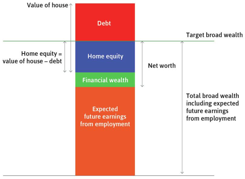
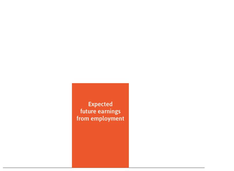
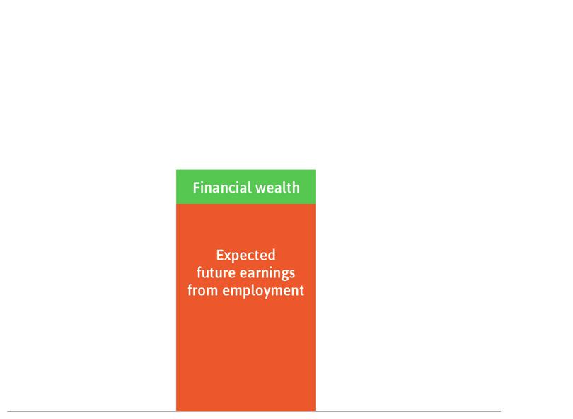
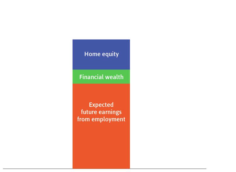
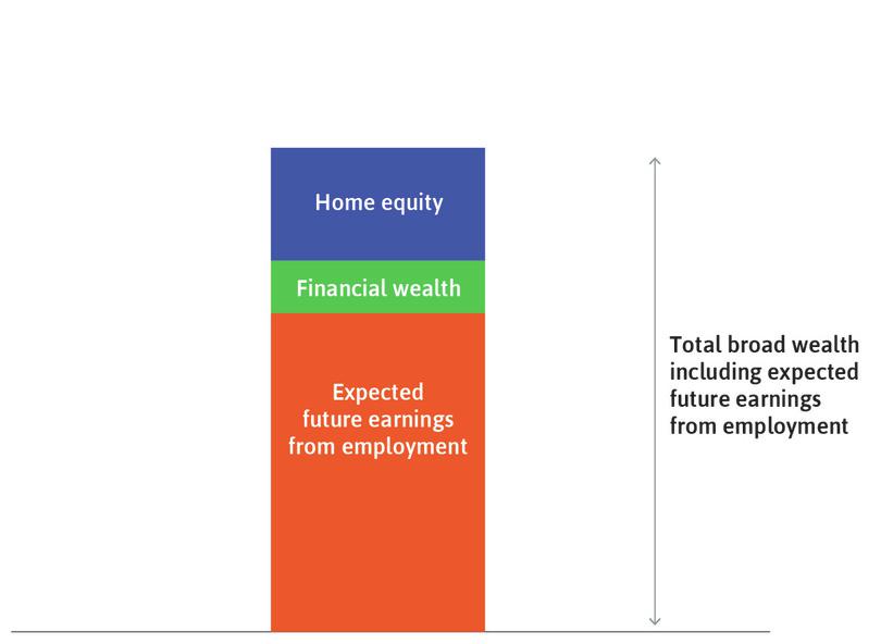
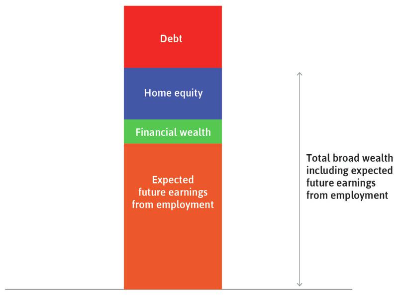
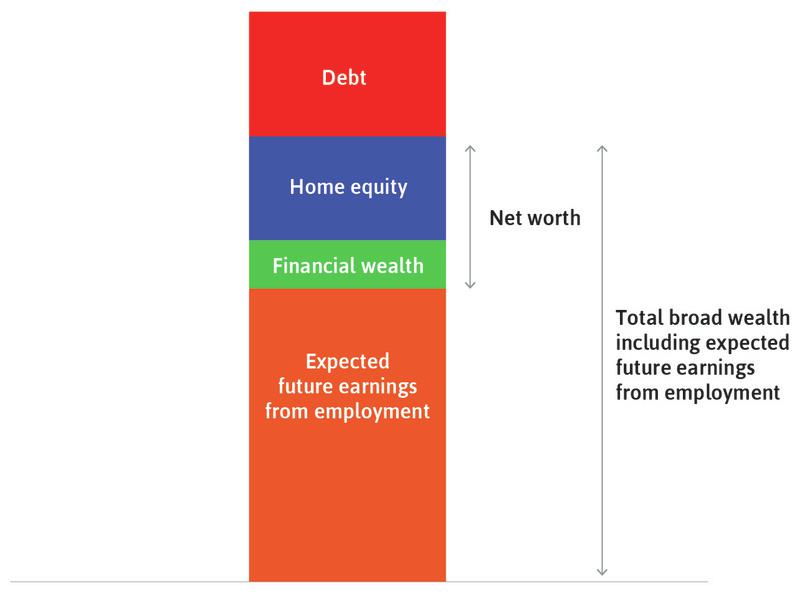
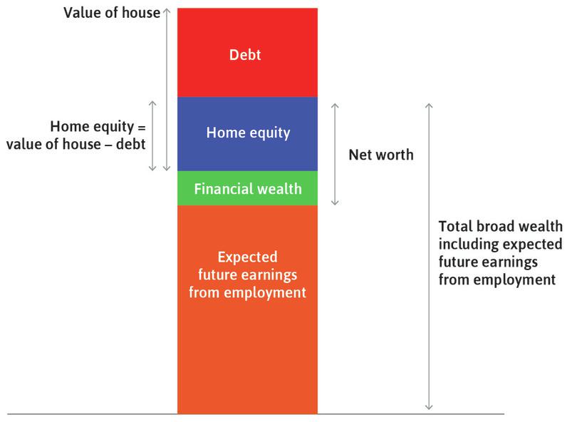
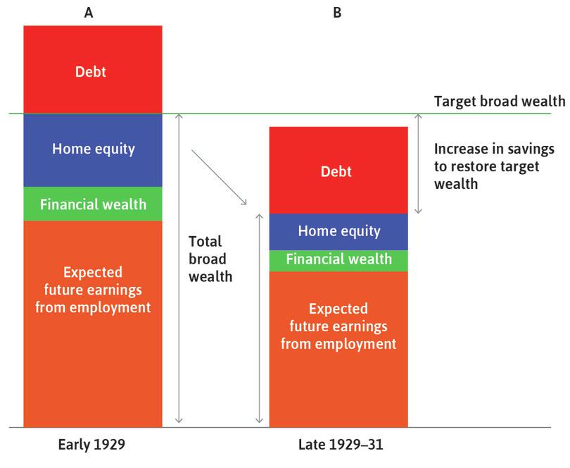
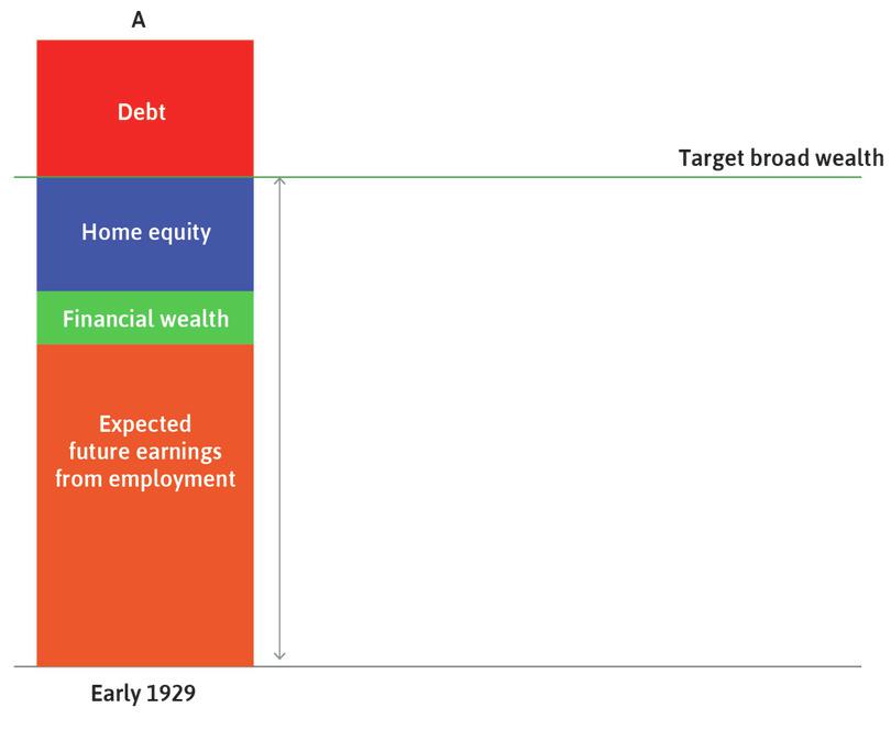
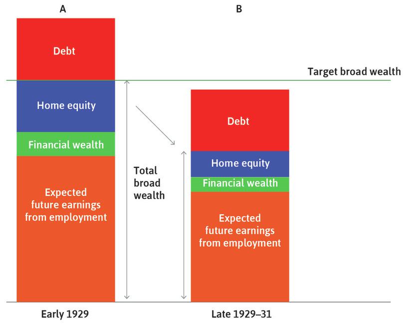
To illustrate why households who were not affected by credit constraints nevertheless cut consumption, we look at the composition of a household’s wealth or assets. In Unit 10 we introduced the concept of wealth by comparing it with the volume of water in a bathtub. At that time we focused on material wealth. In Figure 14.7 we extend the concept of wealth to broad wealth so as to include the household’s expected future earnings from employment, known as the value of its human capital.
Follow the analysis in Figure 14.7 to see the composition of the household’s broad wealth, which is equal to the value of all its assets, minus its debt (which we assume is a mortgage on the house).
- equity
- An individual’s own investment in a project. This is recorded in an individual’s or firm’s balance sheet as net worth. See also: net worth. An entirely different use of the term is synonymous with fairness.
As we shall see:
- If target wealth is above expected wealth: The household will increase savings and decrease consumption.
- If target wealth is below expected wealth: The household will decrease savings and increase consumption.
In early 1929, how would a household with the wealth position shown in column A of Figure 14.8 have interpreted news about factory closures, the collapse of the stock market, and bank failures? How would it have adjusted spending on consumer durables, housing, and non-durables? Answers to these questions help tell us why the Great Depression happened.
- financial accelerator
- The mechanism through which firms’ and households’ ability to borrow increases when the value of the collateral they have pledged to the lender (often a bank) goes up.
- Before the Depression: Viewed from early in 1929 (column A in Figure 14.8), households are shown as making consumption decisions in line with their expectations: total wealth is equal to target wealth.
- The Depression: By late 1929 (column B), the downturn was underway and beliefs had changed. With job losses throughout the economy, households revised expected earnings downward. Falling asset prices (of shares and houses) reduced the value of the household’s material wealth. The result was a gap between the household’s target wealth and expected wealth. This helps to explain the cutback in consumption by households who could (and in an ordinary downturn, would) have helped to smooth a temporary fall in aggregate demand. Instead, these households increased their saving. This fall in autonomous consumption is part of the explanation for the downward shift of the aggregate demand curve from crisis to trough in Figure 14.6.
- The financial accelerator, collateral, and credit constraints: Changes in household wealth affect consumption through another channel. In Unit 10, we saw that having collateral may enable a household to borrow. An important example is the case of home loans, where the bank extends a loan using the value of the house as collateral. If the value of your house falls, the bank will be willing to lend less, making you more credit-constrained, which may reduce your consumption.
The same mechanisms are at work if house prices increase, which will tend to increase consumption:
- For those who are not credit-constrained: If the value of your house increases, this improves your net worth and raises your wealth relative to target. We would predict that this would reduce your precautionary savings, increasing consumption.
- For those who are credit-constrained: A rise in the price of your house can lead you to increase your consumption spending because the higher collateral enables you to borrow more.
Exercise 14.1 A household’s balance sheet
Consider a family of two parents and two children who have a mortgage on their home. They have paid off half the mortgage. The family also owns a car and a portfolio of shares in companies. They spend their income on food, clothing, and private school fees, and have retirement savings held in a pension fund.
- Which of these items would be on a balance sheet for the household?
- Using the example of the bank’s balance sheet in Figure 10.16 as a guide, construct an annual balance sheet for your hypothetical household. You may want to research the typical values for these items for a family of this type.
Exercise 14.2 Housing in France and Germany
In France and Germany, it is difficult for a household to increase its borrowing based on an increase in the market value of the house. In addition, large down-payments (as a percentage of the house price) are required for house purchases.
- On the basis of this information, how would you expect a rise in house prices in France or Germany to affect spending by households?
- In the US or UK, loans are more easily available based on a rise in home equity and only a small down-payment is required. How would you expect your answer to question 1 to change when considering the US or UK?
- What do you conclude about the role of the financial accelerator in France and Germany compared with the UK and the US?
Note: A December 2014 VoxEU article, ‘Combatting Eurozone deflation: QE for the people’, tells you more about the influence of a change in house prices on spending in Europe and the US.
Question 14.3 Choose the correct answer(s)
Which of the following statements is correct regarding household wealth?
- The material wealth is the net worth, that is, financial wealth plus value of house minus its debt.
- This is the definition of broad wealth.
- A household adjusts its precautionary saving in response to the gap (positive or negative) between its actual and target wealth.
- If the target wealth is above its expected wealth, then the household will increase its savings to fill the gap, reducing its consumption as a result.
14.4 Investment spending
In Unit 13, we contrasted the volatility of investment with the smoothness of consumption spending. But how do firms make investment decisions? Think of the manager or owner of a firm deciding what to do with their accumulated profits. There are four choices:
- Dividends: Allocate the funds to managerial or employee salaries, or to dividends for owners.
- Saving: Buy an interest-bearing financial asset such as a bond, or retire (pay off) existing debt.
- Investment abroad: Build new productive capacity in another country.
- Investment at home: Build new capacity in the home country.
The fourth choice is called investment in our model (the third choice is also investment, but since it is spent in the foreign country it is measured in the foreign country’s national accounts as part of its I, not in the home country’s).
If we assume that there is no reason to change salaries then we can also break down the owner’s decision as we did Marco’s decision in Unit 10:
- The owner has the choice to consume now or consume later: Taking the revenue as dividends means the owner can, if desired, simply consume the extra income now.
- If the decision is to consume later: The owner can either save (lend by buying a financial asset such as a bond or retire debt) or invest in a new project.
- If the decision is to invest: Whether the owner does it in the home country or abroad will depend on the expected rate of profit for the potential investment projects in the two locations.
The desirability of consuming more now rather than later depends on the owner’s discount rate (ρ), as discussed in Unit 10. The owner will compare this to the return they can get by not consuming now. If the firm saves by buying a financial asset then the return is the interest rate r. If the firm invests in productive capacity then the return will be the profit rate on investment, which we will call Π as in Unit 10:
- If ρ is greater than both r and Π: The owner will keep the funds and increase consumption spending.
- If r is greater than ρ and Π: The decision will be to repay debt or purchase a financial asset.
- If Π is greater than ρ and r: The owner will invest (either at home or abroad).
- monetary policy
- Central bank (or government) actions aimed at influencing economic activity through changing interest rates or the prices of financial assets. See also: quantitative easing.
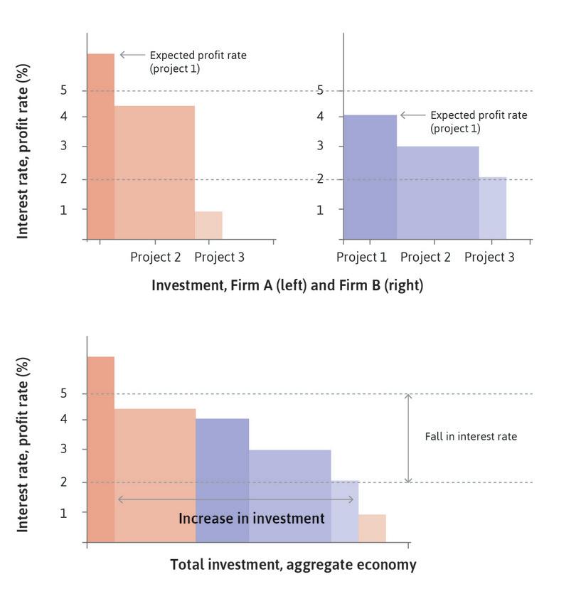
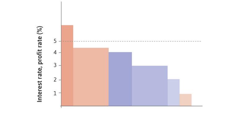
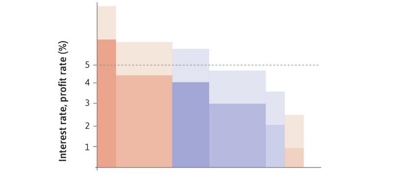
Because of these options, the interest rate is one of the factors determining whether investment takes place. We saw in Unit 10 that this can be altered by central bank policy (monetary policy). The interest rate is the opportunity cost of purchases of machinery, equipment, and structures that increase the capital stock—if you have money available, you could save it with a return of r instead of investing it. Alternatively, if you do not have money available, then the cost of borrowing for investment is also r. If we rank investment projects by their expected post-tax rate of profit, then a lower interest rate raises the number of projects for which the expected rate of profit is greater than the interest rate. We saw this when Marco faced the decision of whether or not to invest (Figure 10.10). Thus a higher interest rate reduces investment, and a lower interest rate increases it.
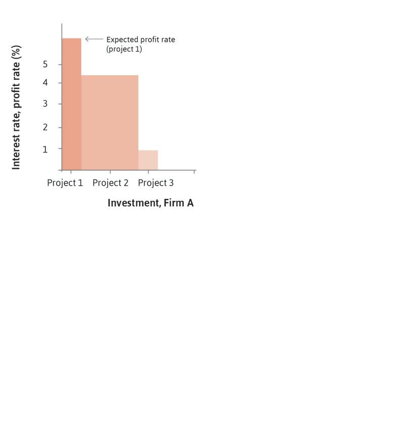
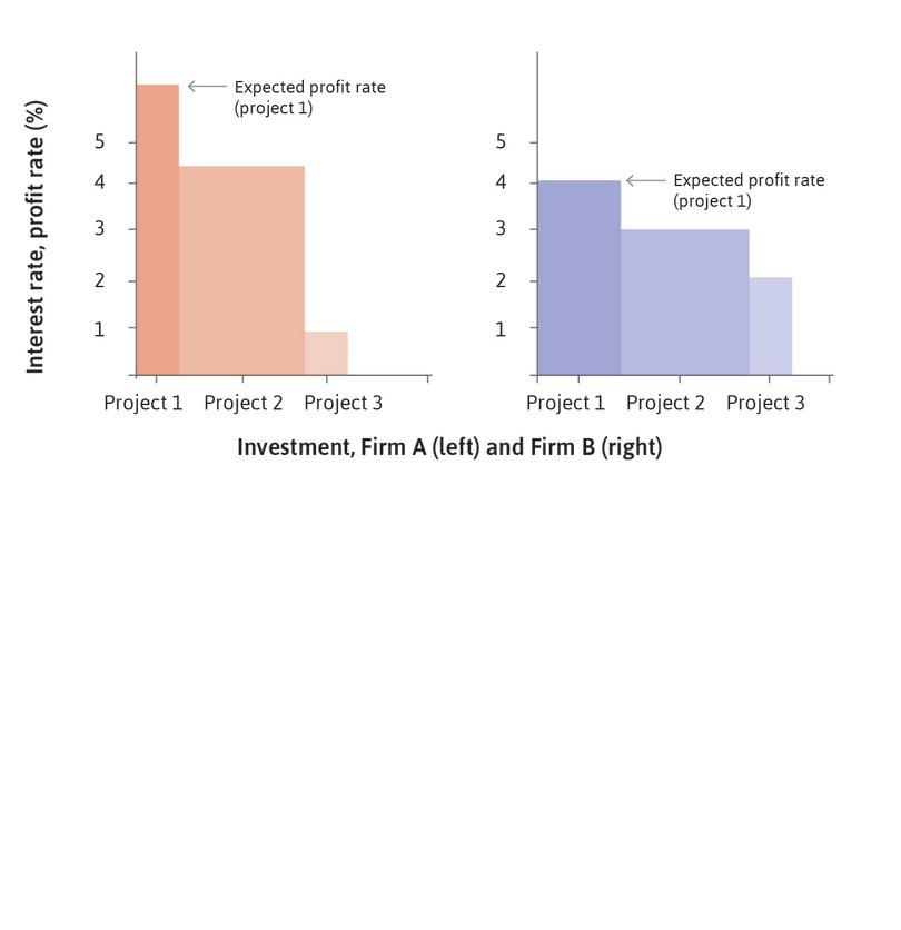
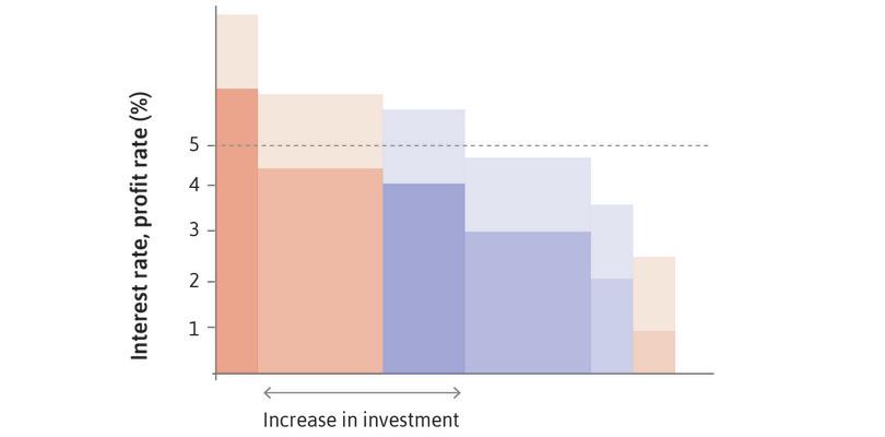
Figure 14.9 illustrates this fact for an economy consisting of two firms, A and B. For each firm in this example, there are three investment projects of different scale and rate of return. They are shown in decreasing order of the expected rate of profit. Follow the analysis in Figure 14.9 to see how the interest rate determines which investment projects go ahead. The lower panel aggregates the two firms to show how investment in the economy as a whole responds to a change in the interest rate.
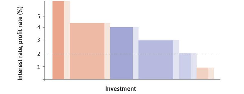
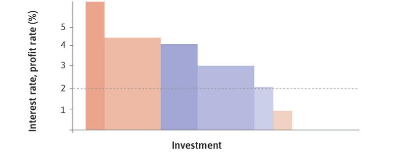
In Figures 14.10a–c, we look at how a change in profit expectations affects investment.
In the two-firm economy in Figure 14.10a, the expected rate of profit for each project rises because of an improvement in the supply-side conditions in the economy. The height of each column rises, and as a result, there is more investment at a given interest rate.
An upward shift can be caused by a fall in expected input prices, such as a forecast fall in the price of energy or wages, or a fall in taxation over the life of the project.
- expropriation risk
- The probability that an asset will be taken from its owner by the government or some other actor.
Another example of a positive supply effect is an improvement in the security of property rights so that there is a smaller chance that the government or another powerful actor (such as a landowner, like Bruno in Unit 5, who might threaten a smallholder) will take over ownership of the investment project. This is called a fall in the risk of expropriation and is an example of an improvement in the business environment.
In Figure 14.10b, the height of the columns remains unchanged, but their width (representing the amount of investment that is profitable in many projects) has increased. This is the result of a permanent increase in demand and the lack of sufficient capacity to meet forecast sales.
- investment function (aggregate)
- An equation that shows how investment spending in the economy as a whole depends on other variables, namely, the interest rate and profit expectations. See also: interest rate, profit.
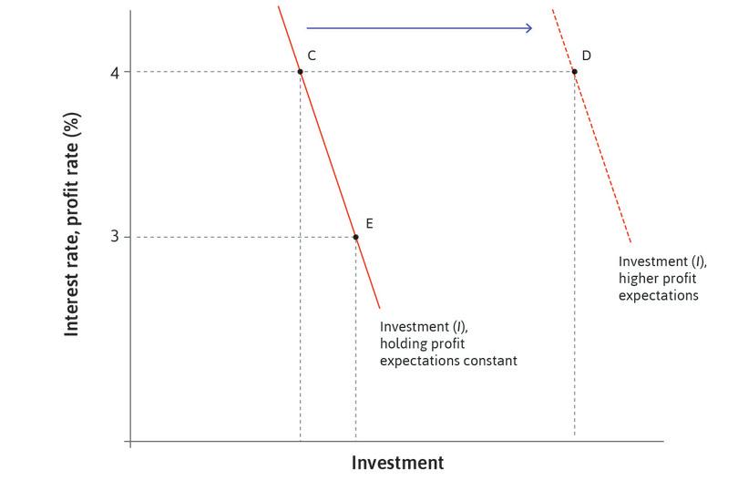
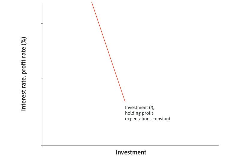
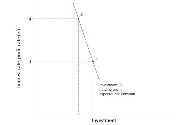
In an economy with many thousands of firms, a downward-sloping line (as in Figure 14.10c) represents the potential investment projects. This is called the aggregate investment function. The response of investment to a change in the interest rate is shown as a shift from C to E. Figure 14.10c also shows the effect of a change in the profitability of investment, which arises from supply and demand effects and raises investment from C to D for the same interest rate.
The empirical evidence suggests that business spending on machinery and equipment is not very sensitive to the interest rate. The limited effect of changes in the interest rate on business investment (illustrated by the steepness of the lines in the figure) highlights the importance of the supply- and demand-side factors that shift the investment function (Figures 14.10a and 14.10b).
The interest rate affects investment spending outside the business sector through its effects on households’ decisions to purchase new or larger homes, which influence new housing construction. The interest rate also has substantial effects on the demand for durable consumer goods, such as cars and home appliances, which are often purchased using credit.
Question 14.4 Choose the correct answer(s)
Figure 14.9 depicts possible investment projects for Firms A and B.
Based on this information, which of the following statements is correct?
- For Firm B, the expected profit rate from its project 1 is less than 5%. Therefore only Firm A undertakes its project 1.
- At an interest rate of 1.5%, Firm A will not undertake project 3.
- With a permanent positive demand shock, the heights of the columns remain unchanged but the amount of investment that is profitable increases. This increases the widths of the columns, leading to higher investment (for any given interest rate).
- The fall in energy prices reduces costs for firms so expected profits increase, implying that more projects have an expected profit rate greater than the interest rate.
Question 14.5 Choose the correct answer(s)
Figure 14.10c depicts the aggregate investment function of an economy.
Based on this information, which of the following statements is correct?
- The investment line represents the relationship between investment and interest rate, ceteris paribus. Therefore the fall in investment would be shown by a movement up the original line (from E to C for example), not a shift of the line.
- A rise in corporate tax would decrease the expected profit rate, shifting the investment line inwards. This results in a fall in investment.
- Higher demand makes it profitable to invest in larger projects, increasing investment at a given interest rate.
- A steeper line means smaller changes in investment when the interest rate moves, that is, lower sensitivity of investment to the interest rate.
14.5 The multiplier model: Including the government and net exports
Here we add governments and central banks to the model so that we can show how they can stabilize (or destabilize) the economy after a shock. As before, we assume that firms are willing to supply any amount of goods demanded, so:
We saw in Unit 13 that when we include the government and interactions with the rest of the world through exports and imports, aggregate demand can be split into these components:
To understand the aggregate demand function as shown above, it is useful to go through each component in turn:
Consumption
Household consumption spending depends on post-tax income. The government charges a tax t, which we assume is proportional to income. The income left after the payment of tax, (1 − t)Y, is called disposable income. The marginal propensity to consume, c1, is the fraction of disposable income (not pre-tax income) consumed. This means that in the aggregate consumption function:
- Spending on consumption is written as: C = c₀ + c1(1 − t)Y.
- All of the influences on consumption apart from current disposable income are included in autonomous consumption, c₀, and will therefore shift the consumption function in the multiplier diagram. These include wealth and target wealth, collateral effects, and changes in the interest rate.
Investment
We have just seen that investment spending will be influenced by the interest rate and the expected post-tax rate of profit. In the aggregate investment function:
- Spending on investment is a function of the interest rate and the expected post-tax rate of profit.
- Ceteris paribus, a higher interest rate reduces investment spending, shifting down the aggregate demand curve.
- A higher expected post-tax rate of profit raises investment spending, shifting up the aggregate demand curve.
Government spending
- exogenous
- Coming from outside the model rather than being produced by the workings of the model itself. See also: endogenous.
Much of government spending (excluding transfers) is on general public services, health, and education. Government spending does not change in a systematic way with changes in income. It is referred to as exogenous.
An increase in government spending shifts the aggregate demand curve up in the multiplier diagram.
Net exports
- marginal propensity to import
- The change in total imports associated with a change in total income.
The home economy sells goods and services abroad, which are its exports. The amount of foreign goods the home economy demands (its imports) will depend on domestic incomes. The fraction of each additional unit of income that is spent on imports is termed the marginal propensity to import (m), which must be between 0 and 1. So we have:
- exchange rate
- The number of units of home currency that can be exchanged for one unit of foreign currency. For example, the number of Australian dollars (AUD) needed to buy one US dollar (USD) is defined as number of AUD per USD. An increase in this rate is a depreciation of the AUD and a decrease is an appreciation of the AUD.
If a country’s costs of production fall so that it can sell its goods at a lower price on world markets compared to the prices of other countries, the demand for its exports will increase, and domestic demand for imports will fall. We will see in the next unit that the exchange rate affects the prices of a country’s goods on world markets. Growth in world markets also increases exports. For now, however, we will ignore these effects and assume that exports are also exogenous.
Putting together each of the components of aggregate demand we have:
Both taxes and imports reduce the size of the multiplier. Recall that the multiplier tells us the amount by which an increase in spending (such as a rise in autonomous consumption, investment, government spending, or exports) raises GDP in the economy. When we include taxation and imports in the model, the indirect multiplier effect of a given rise in spending on GDP is smaller. This is because some household income goes straight to the government as taxation, and some is used to buy goods and services produced abroad. Because we assume that the government does not increase its spending when taxes go up, and foreign buyers do not import more of our goods when we import more of theirs, this means that some of an autonomous increase in income does not lead to further indirect increases in income in the domestic economy. Like saving, taxation and imports are referred to as leakages from the circular flow of income. The result is to reduce the indirect effects of an autonomous change in spending on aggregate demand, output, and employment.
To summarize:
- A higher marginal propensity to import reduces the size of the multiplier: This makes the aggregate demand curve flatter.
- An increase in exports shifts the aggregate demand curve up in the multiplier diagram.
- An increase in the tax rate reduces the size of the multiplier: This makes the aggregate demand curve flatter.
The Einstein at the end of this section shows you how to calculate the size of the multiplier in the model once the tax rate and imports are included. To illustrate, we assume a tax rate of 20% (0.2) and a marginal propensity to import of 0.1. Before we introduced the government, we set the marginal propensity to consume, c1, at 0.6. If we use these numbers in the formula for the multiplier that we calculate in the Einstein, we get the result that the value of the multiplier is k = 1.6, compared to 2.5 without including taxation and imports. In the next section we look at how economists have estimated the size of the multiplier from data, why their estimates differ, and why it matters.
Exercise 14.3 The multiplier model
Consider the multiplier model discussed above.
- Compare two economies, which differ only in their share of credit-constrained households but are identical otherwise. In which economy is the multiplier larger? Illustrate your answer using a diagram.
- On the basis of your comparison of the two economies, would you expect the multiplier in an economy to vary over its business cycle?
- Some economists estimated the size of the multiplier in the Great Depression to be equal to 1.8. Explain how the following characteristics of the US economy at the time could have affected its value:
- the size of government (see Figure 14.1)
- the fact that there were no unemployment benefits
- the fact that the share of imports was small
Question 14.6 Choose the correct answer(s)
The aggregate demand of an open economy is given by the after-tax domestic consumption C, the investment I (which depends on the interest rate r), the government spending G and net exports X − M:
c₀ is autonomous consumption, c₁ is the marginal propensity to consume, and m is the marginal propensity to import. In the economy’s equilibrium this equals its output: AD = Y. Solving for Y yields:
Given this equation, which of the following increases the multiplier?
- G affects the level of AD but not the multiplier.
- r affects I(r), which in turn affects the level of AD but not the multiplier.
- A fall in m increases the multiplier. This is because it reduces leakages in the economy.
- A rise in t reduces the multiplier.
Einstein The multiplier in an economy with a government and foreign trade
We can again use the fact that there is equilibrium in the goods market when output is equal to aggregate demand to find the multiplier (equilibrium is where the aggregate demand line crosses the 45-degree line in the multiplier diagram). The aggregate demand equation can be rearranged to solve for output and consequently the multiplier:
Therefore:
We can see that the multiplier is smaller when we introduce the government and foreign trade:
The reason is that the denominator on the left-hand side is larger than on the right:
14.6 Fiscal policy: How governments can dampen and amplify fluctuations
There are three main ways that government spending and taxation can dampen fluctuations in the economy:
- The size of government: Unlike private investment, government spending on consumption and investment is usually stable. Spending on health and education, which are the two largest government budget items in most countries, does not fluctuate with capacity utilization or with business confidence. These kinds of government spending stabilize the economy. As we have also seen, a higher tax rate dampens fluctuations because it reduces the size of the multiplier.
- The government provides unemployment benefits: Although households save to smooth fluctuations in income, few households save enough (that is, self-insure) to cope with an extended period of unemployment. So unemployment benefits help households to smooth consumption. Other programs to redistribute income to the poor have the same smoothing effect.
- The government can intervene: It can intervene deliberately to stabilize aggregate demand using fiscal policy.
- fiscal policy
- Changes in taxes or government spending in order to stabilize the economy. See also: fiscal stimulus, fiscal multiplier, aggregate demand.
- co-insurance
- A means of pooling savings across households in order for a household to be able to maintain consumption when it experiences a temporary fall in income or the need for greater expenditure.
- hidden actions (problem of)
- This occurs when some action taken by one party to an exchange is not known or cannot be verified by the other. For example, the employer cannot know (or cannot verify) how hard the worker she has employed is actually working. Also known as: moral hazard. See also: hidden attributes (problem of).
Could workers insure privately against job loss? There are also three reasons why the private market fails, and therefore governments provide unemployment insurance in the form of unemployment benefits:
- Correlated risk: In a recession, job loss will be widespread. This means that there will be a surge in insurance claims across the economy and a private provider may be unable to pay out on the scale required. It also means co-insurance among a group of neighbours or family members may be of limited use, as the need for help may arise in many households at the same time.
- Hidden actions: As we saw in Unit 12, the insurance company cannot observe the reason for the job loss so it would have to insure the employee against a firm cutting back employment due to lack of demand, as well as the worker being fired for inadequate work. This creates a moral hazard, because a well-insured person is expected to make less of an effort on the job.
- Hidden attributes: Suppose you learn that your firm is in difficulty, but the insurance company does not. This is another example of asymmetric information. You will therefore buy insurance when you learn of the likely closure of the firm, and it will be provided at good rates because the insurance company does not know that you are likely to make a claim on them. Workers who know their firm is performing well will not buy insurance. The hidden attributes problem will be true about individuals (hardworking or lazy), as well as firms (successful or failing). The good prospects (those who enjoy working hard, for example) will shun the insurance and the insurer will be left with those likely to face the extra risks of losing their job.
The system of unemployment benefits is part of the automatic stabilization that characterizes modern economies. We have already seen another automatic stabilizer: a proportional tax system reduces the size of the multiplier and dampens the business cycle.
- moral hazard
- This term originated in the insurance industry to express the problem that insurers face, namely, the person with home insurance may take less care to avoid fires or other damages to his home, thereby increasing the risk above what it would be in absence of insurance. This term now refers to any situation in which one party to an interaction is deciding on an action that affects the profits or wellbeing of the other but which the affected party cannot control by means of a contract, often because the affected party does not have adequate information on the action. It is also referred to as the ‘hidden actions’ problem. See also: hidden actions (problems of), incomplete contract, too big to fail.
- hidden attributes (problem of)
- This occurs when some attribute of the person engaging in an exchange (or the product or service being provided) is not known to the other parties. An example is that the individual purchasing health insurance knows her own health status, but the insurance company does not. Also known as: adverse selection. See also: hidden actions (problem of).
- asymmetric information
- Information that is relevant to the parties in an economic interaction, but is known by some but not by others. See also: adverse selection, moral hazard.
- automatic stabilizers
- Characteristics of the tax and transfer system in an economy that have the effect of offsetting an expansion or contraction of the economy. An example is the unemployment benefits system.
- paradox of thrift
- If a single individual consumes less, her savings will increase; but if everyone consumes less, the result may be lower rather than higher savings overall. The attempt to increase saving is thwarted if an increase in the saving rate is unmatched by an increase in investment (or other source of aggregate demand such as government spending on goods and services). The outcome is a reduction in aggregate demand and lower output so that actual levels of saving do not increase.
- fallacy of composition
- Mistaken inference that what is true of the parts (for example a household) must be true of the whole (in this case the economy as a whole). See also: paradox of thrift.
In our list, the third role of government in dampening fluctuations is the use of fiscal policy in deliberate stabilization policies: an increase in government spending or cuts in taxation to support aggregate demand in a downturn; or trimming spending and raising taxes to rein in a boom. It can be cumbersome to have these fiscal policy measures approved by a parliament, which has power over budgetary decisions, which is one reason why stabilization policy is often handled through monetary, rather than fiscal, policy. But fiscal policy can also play an important role in stabilization, as we now consider, especially in particularly large downturns.
The paradox of thrift and the fallacy of composition
By comparing a household with the economy as a whole, we better understand the nature of an increase in the government’s deficit in a recession. Faced with a household budget deficit, a family worried about their falling wealth cuts spending and saves more. We saw exactly this behaviour in Figure 14.8 when households increased their savings in 1929. Keynes showed that the wisdom of family precautionary saving does not apply to the government when the economy is in a recession.
Compare the attempt to save more by a single household and by all households in the economy simultaneously. Think of a single household cutting expenditures and putting its additional savings in a sock. The money is in the sock for when the household decides it is wise to spend it.
Now, assume that all households cut expenditures and put additional savings in their socks. Assuming nothing else in the economy changes, the additional saving causes lower aggregate consumption spending in the economy. What happens? From the previous section, we can model this as a fall in autonomous consumption, c₀: the aggregate demand curve shifts down. The economy moves through the multiplier process to a lower level of output, income, and employment. The aggregate attempt to increase savings led to a fall in aggregate income, which is known as the paradox of thrift. The fact that what is true for one part of the economy is not true of the whole economy is known as the fallacy of composition.
A single household can increase its savings if it anticipates bad luck, and the saving will be there if it is unlucky—for example, if someone becomes ill or loses a job. However, if every household does this when the economy is in a recession, this behaviour causes the bad luck: more people lose their jobs. The reason is that in the economy as a whole, spending and earning go together. My spending is your income. Your spending is my income.
What can be done? The government can allow the automatic stabilizers to operate and help absorb the shock. In addition, it can provide an economic stimulus (such as a temporary increase in government spending or a temporary cut in taxation) until business and consumer confidence return and the private sector regains its willingness to spend. Budget deficits rise, but this avoids a deep recession, as Keynes realized.
- fiscal stimulus
- The use by the government of fiscal policy (via a combination of tax cuts and spending increases) with the intention of increasing aggregate demand. See also: fiscal multiplier, fiscal, policy, aggregate demand.
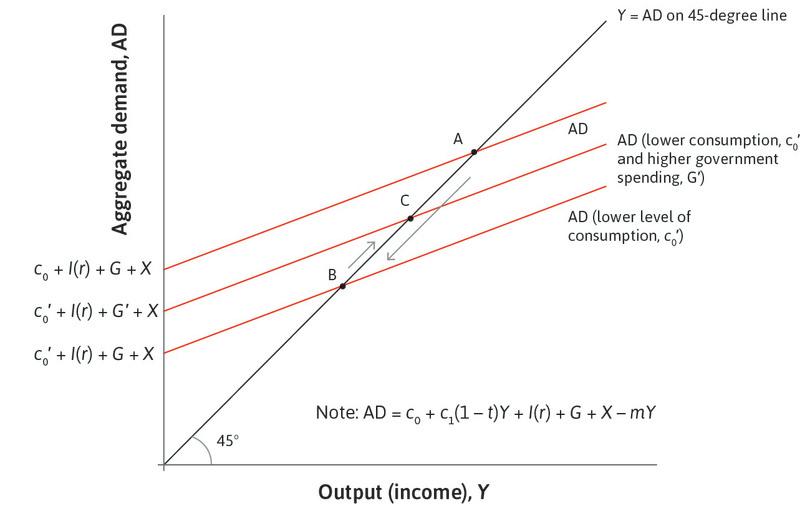
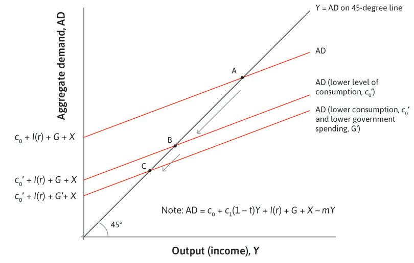
When a government cuts taxes or increases government spending G in a recession, it is called a fiscal stimulus. The aim is to counteract the fall in aggregate demand from the private sector. A tax cut is intended to encourage the private sector to spend more, while an increase in G is a direct addition to aggregate demand. Figure 14.11a shows how an increase in G can offset a decline in private consumption, such as that described by the paradox of thrift. Like an exogenous increase in investment, the rise in G operates via the multiplier, so the increase in output will typically be greater than the increase in G.
Great economists John Maynard Keynes
John Maynard Keynes (1883–1946) and the Great Depression of the 1930s changed the course of economic thought. Until then, most economists had seen unemployment as the result of some kind of imperfection in the labour market. If this market worked optimally it would equate the supply of, and demand for, workers. The massive and persistent unemployment in the decade prior to the Second World War led Keynes to look again at the problem of joblessness.
Keynes was born into an academic family in Cambridge, UK. He studied mathematics at King’s College, Cambridge and then became an economist and prominent follower of the renowned Cambridge professor, Alfred Marshall. Before the First World War, Keynes was a world authority on the quantity theory of money and the gold standard, and held conservative views on economic policy, arguing for a limited role of government. But his views would soon change.
In 1919, following the end of the First World War, Keynes published The Economic Consequences of the Peace, which opposed the Versailles settlement that ended the war.2 This book instantly made him a global celebrity. Keynes rightly argued that Germany could not pay large reparations for the war, and that an attempt to make Germany do this would help provoke a worldwide economic crisis. In 1925, Keynes opposed Britain’s return to the gold standard, arguing that this policy would lead to a contraction of the economy. In 1929 there was a financial crash and global crisis. The Great Depression followed. In 1931 Britain was driven off the gold standard.
In response to these dramatic events, Keynes explained that the orthodox monetary policies required by the gold standard would worsen the depression, and that the world needed policies to increase aggregate demand. In 1936, he published The General Theory of Employment, Interest and Money in which he set out an economic model to explain these views.3 The General Theory immediately became world famous, particularly for the idea of the multiplier, which is explained in this unit. In The General Theory, Keynes reasoned that if interest rates were already very low, then fiscal expansion would be necessary to alleviate depression. Such was the lasting influence of his work that the initial response in many countries to the global economic crisis of 2008 was to apply such Keynesian policies.
During the Second World War, Keynes turned to postwar reconstruction, determined to ensure that the mistakes that followed the First World War would not be repeated. In 1944, with Harry Dexter White of the US, he led an international conference at Bretton Woods in New Hampshire that resulted in the creation of a new international monetary system, managed by the International Monetary Fund, or IMF. The Bretton Woods system was designed to avoid the mistakes Keynes had unsuccessfully warned against in the aftermath of the First World War, and to ensure that a country that was in recession (and had balance of payments difficulties) would not need to follow the contractionary policies required by the gold standard. A country like this could use fiscal policy to pursue full employment, while at the same time it could devalue its exchange rate to encourage exports, reduce imports, and achieve a satisfactory balance of payments position.
Keynes led a remarkably varied life. He was an academic, a senior civil servant, owner of the New Statesman magazine, financial speculator, chairman of an insurance company, and member of the British House of Lords. He was also the founder of the Arts Council of Great Britain and chairman of the Covent Garden Opera Company. He was married to the Russian ballerina Lydia Lopokova and was a key member of the Bloomsbury Group, a remarkable circle of artistic and literary friends in London, which included the novelist Virginia Woolf.
In 1926, in a pamphlet entitled The End of Laissez-Faire,4 he wrote:
For my part I think that capitalism, wisely managed, can probably be made more efficient for attaining economic ends than any alternative system yet in sight, but that in itself it is in many ways extremely objectionable. Our problem is to work out a social organization which shall be as efficient as possible without offending our notions of a satisfactory way of life.
How governments can amplify fluctuations
Keynes’ argument refers to the cell in the bottom right of Figure 14.12 at the end of this section: poor policymaking that amplifies the business cycle.
- government budget balance
- The difference between government tax revenue and government spending (including government purchases of goods and services, investment spending, and spending on transfers such as pensions and unemployment benefits). See also: government budget deficit, government budget surplus.
- government budget deficit
- When the government budget balance is negative. See also: government budget balance, government budget surplus.
- government budget surplus
- When the government budget balance is positive. See also: government budget balance, government budget deficit.
Sometimes a government chooses to raise taxes or cut spending during a recession because it is concerned about the effect of a recession on its budget balance. The government budget balance is the difference between government revenue less transfers, T, and government spending, G, that is, (T − G). As we have seen, if the economy is in recession, government transfers, like unemployment benefits, rise while tax revenues fall, so the government’s budget balance deteriorates and may become negative.
When the government’s budget balance is negative, this is called a government budget deficit—government spending on goods and services, including investment spending, plus spending on transfers (such as pensions and unemployment benefits) is greater than government tax revenue. A government budget surplus is when tax revenue is greater than government spending. To summarize:
- Budget in balance: G = T
- Budget deficit: G > T
- Budget surplus: G < T
The worsening of the government’s budgetary position in a recession is part of its stabilizing role. Conversely, when the government chooses to override the stabilizers to reduce its deficit, this may amplify fluctuations in the economy.
Suppose a government tries to improve its budgetary position in a recession by cutting its spending. This, like a tax increase, is referred to as austerity policy. Follow the analysis in Figure 14.11b to see how austerity policy can reinforce a recession by further reducing aggregate demand.
Does this argument mean that governments should never impose austerity in order to reduce a fiscal deficit? No—just that a recession is not a wise time to do it. Running government deficits under the wrong economic conditions can be harmful. In a well-designed policy framework, there will be constraints on government action, as we will see in Section 14.8.
- negative feedback (process)
- A process whereby some initial change sets in motion a process that dampens the initial change. See also: positive feedback (process).
- positive feedback (process)
- A process whereby some initial change sets in motion a process that magnifies the initial change. See also: negative feedback (process).
The table in Figure 14.12 summarizes the lessons so far. The first row gives examples of how household behaviour may either smooth or disrupt the economy. The terms negative and positive feedback are used to refer to dampening and amplifying mechanisms in the business cycle.
| Dampening mechanisms offset shocks (stabilizing) | Amplifying mechanisms reinforce shocks (may be destabilizing) | |
|---|---|---|
| Private sector decisions |
|
|
| Government and central bank decisions |
|
|
The role of the private sector and the government in the business cycle.
Figure 14.12 The role of the private sector and the government in the business cycle.
Exercise 14.4 Spending cuts in a recession
Assume the government is initially in budget balance.
- Does the government’s budget balance improve, deteriorate, or remain unchanged if the government cuts its spending in a recession, ceteris paribus? To answer this question, use the example in Figure 14.11b. Assume the budget was in balance at point A. Once at B, the government cuts G in an attempt to improve its budget balance. Assume there are no unemployment benefits and a linear tax.
- Evaluate the government’s policy.
Question 14.7 Choose the correct answer(s)
Which of the following statements is correct?
- If the government maintains fiscal balance then it is not offsetting the decline in private demand.
- Automatic stabilizers refer to government policies that smooth household disposable incomes, such as taxes and unemployment benefits.
- The multiplier as we have defined it so far assumes that there is spare capacity in the economy. It will be low or zero if there is little or no spare capacity.
- A rise in G increases aggregate demand directly while a cut in taxes can increase C and/or I, representing increased private sector demand.
14.7 The multiplier and economic policymaking
In the multiplier model, we have used simple ways of modelling aggregate consumption, investment, trade, and government fiscal policy. This means there are a small number of variables from which the size of the multiplier is calculated (the marginal propensity to consume, the marginal propensity to import, and the tax rate). When we apply the model to the real world, it is important to realize that there is no single multiplier that applies at all times.
Crowding out
The effect of an increase in government spending in reducing private spending, as would be expected for example in an economy working at full capacity utilization, or when a fiscal expansion is associated with a rise in the interest rate.
The multiplier will be a different size if the economy is operating at full capacity utilization and low unemployment than in a recession. With fully employed resources, a 1% increase in government spending would displace or crowd out some private spending in the economy. To consider an extreme case, if all workers are employed, then an increase in government employment can only come about by taking workers out of the private sector. If increased government production were offset exactly by reduced private sector production, then the multiplier would be zero.
We would not normally expect a government to undertake a fiscal expansion when unemployment is very low—although it may in exceptional circumstances like war, as the US did in the later years of the Second World War and in the Vietnam War.
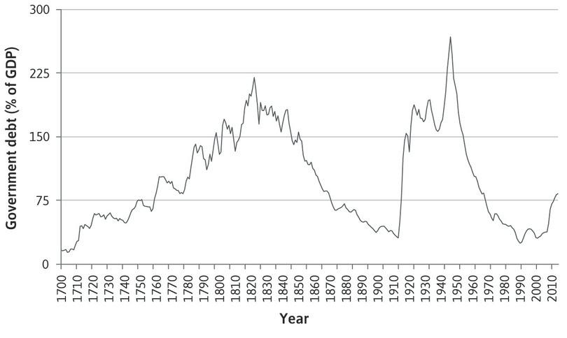
The size of the multiplier will also depend on the expectations of firms and businesses. The economy is not like a bicycle tyre, from which air can be pumped in or let out to keep the pressure at the right level. Households and firms react to policy changes, but they also anticipate them. For example, if firms anticipate that the government will stabilize the economy following a negative shock, this will support business confidence, and the policymaker will be able to use a smaller stimulus. Alternatively, if households think that higher government spending will be followed by higher taxes, those who have the ability to save may put aside more of their money to pay the extra taxes. If this happened, it would reduce the impact of the stimulus.
When the financial crisis in 2008 led to the biggest fall in GDP in many economies since the Great Depression, the world’s policymakers expected an answer from economists: would fiscal policy help to stabilize the economy? The multiplier model, inspired by Keynes’ analysis of the Great Depression, suggested that it would. But by 2008, many economists doubted that the Keynesian model was still relevant. The crisis has revived interest in it and has led to a greater, though not complete, consensus among economists about the size of the multiplier (see below).
In 2012 a study published by Alan Auerbach and Yuriy Gorodnichenko, two economists, showed how the multiplier varies in size according to whether the economy is in a recession or in an expansion.5 This is exactly the insight that policymakers needed in 2008.
For the US, their study suggested a $1 increase in government spending in the US raises output by about $1.50 to $2.00 in a recession, but only about $0.50 in an expansion. Auerbach and Gorodnichenko extended their research to other countries and found similar results. They also found that the effect of autonomous increases in spending in one country had spillover effects on the countries with which they trade. These effects were about the same magnitude as the indirect effects of second, third, and further rounds of spending in the home country.
How economists learn from facts The Mafia and the multiplier
- natural experiment
- An empirical study exploiting naturally occurring statistical controls in which researchers do not have the ability to assign participants to treatment and control groups, as is the case in conventional experiments. Instead, differences in law, policy, weather, or other events can offer the opportunity to analyse populations as if they had been part of an experiment. The validity of such studies depends on the premise that the assignment of subjects to the naturally occurring treatment and control groups can be plausibly argued to be random.
- reverse causality
- A two-way causal relationship in which A affects B and B also affects A.
It may surprise you that economists have used the Italian government’s struggle against the Mafia to uncover the size of the multiplier, but that’s what Antonio Acconcia, Giancarlo Corsetti, and Saverio Simonelli were able to do.6 Adopting the natural experiment method to address the problem of reverse causality, they used data on Mafia-related dismissals of local politicians to isolate the variation in public spending that is not caused by variations in output.
After legal changes in 1991, the central government dismissed provincial councils in Italy who were revealed to have close links with the Mafia, and appointed new officials in their place. These technocrats cut local spending by 20% on average. The change in public spending occurred because of the Mafia links, through their effect on the replacement of government officials. And because there is no direct causal link from proximity to the Mafia to the variation in output, proximity to the Mafia can be used to uncover the causal effect of a change in public spending on output. This situation is illustrated in Figure 14.13.
Using this method, the researchers were able to estimate multipliers of 1.5 at the local level.
Economists have used their ingenuity to come up with methods of estimating the size of the multiplier and the implication of its operation for jobs. Using the US stimulus program that was implemented in the wake of the financial crisis (the American Recovery and Reinvestment Act of 2009, a $787 billion fiscal stimulus), we would expect that US states that were more severely hit by the financial crisis would have had higher unemployment and attracted more stimulus spending by the government. So unemployment causes more spending in those states. This makes it difficult to estimate the effect of higher spending on output and unemployment, which is what we want to do if we want to know the size of the multiplier.
One approach to get around this problem of reverse causality is to make use of the fact that some of the spending in the US stimulus program was distributed to US states using a formula that was unrelated to the severity of the recession experienced in each state. For example, some road-repair expenditures funded by the stimulus package were based on the length of highway in each state.7
Given the formula for allocating road-building funds and the fact that more miles of highway has no direct effect on the change in unemployment, this allows us to answer the question: were more jobs created in states that received more stimulus spending?8
The results of studies using this approach estimated a multiplier of 2, and suggest that the American Recovery and Reinvestment Act created between 1 million and 3 million new jobs.
In spite of scepticism among some economists before the 2008 crisis that the multiplier was greater than one, policymakers around the world embarked on fiscal stimulus programs in 2008–09. Fiscal stimulus was credited with helping to avert another Great Depression, as we will see in Unit 17.
When economists disagree How responsive is the economy to government spending?
There are few questions in economic policy discussed as heatedly in the years since the financial crisis in 2008 as the size of the fiscal multiplier: what is the effect on GDP of a 1% increase in government spending?
Much of the heat is generated by political differences among those involved. People who favour greater government expenditure tend to think the multiplier is large, while those who would like a smaller government tend to think that it is small. (We don’t know whether this correlation is because their beliefs about government influence their estimates of the size of the multiplier, or the other way round.)
This debate has been going on since the first theoretical formalization of the multiplier by John Maynard Keynes in the 1930s. The recent economic crisis has revitalized it for two reasons:
- Monetary policy could not be used: Following the financial crisis, several major economies remained in recession despite central banks cutting interest rates to very close to zero. As we will see in the next unit, interest rates cannot be cut below zero, so governments wanted to know if the fiscal stimulus of an increase in government spending would help stabilize the economy.
- Arguments about whether austerity works: After the Eurozone crisis in 2010, many European countries that were in recession adopted austerity measures of cutting government spending, with the objective of bringing their public finances back to balance.
In both stimulus and austerity, the success of the policy depends on the size of the multiplier. If the multiplier is negative—which could happen if a rising fiscal deficit causes a large reduction in confidence—a stimulus package would lead to a reduction in GDP, and an austerity policy would cause GDP to rise. If the multiplier is positive but less than 1, a fiscal stimulus would raise GDP but by less than the increase in government spending. If, as in our multiplier model, the multiplier is greater than 1, a fiscal stimulus would raise GDP by more than the increase in government spending and a policy of austerity would reinforce the recession conditions.
Depending on methodologies and assumptions, economists have put forward different estimates of multipliers, from negative numbers to values greater than 2. For instance, members of President Obama’s Council of Economic Advisors estimated the multiplier as 1.6 when they prepared the American Recovery and Reinvestment Act of 2009. The International Monetary Fund presented estimates in 2012 that multipliers in advanced economies were, after the crisis, between 0.9 and 1.7.9
To be effective, government spending needs to put resources that would otherwise be idle into productive use. These resources can be unemployed (or underemployed) workers, as well as offices, shops, or factories functioning with spare capacity. When an economy functions at full capacity (with no idle resources), extra government spending will crowd out private spending.
Robert Barro and Paul Krugman, the economists, disagreed about the size of the multiplier in the weeks that followed the enactment of the American Recovery and Reinvestment Act in early 2009. Using data on government defence spending during the Second World War, Barro concluded that the multiplier was not larger than 0.8. That is, spending $1 on military equipment yielded only 80 cents of output. However, Krugman responded that in wartime there are no idle productive resources to take advantage of. People of working age were in work supporting the war effort in factories, and the government used rationing to depress private consumption.10
In the recessions that followed the Eurozone crisis in 2010, just as new economic research was finding evidence that multipliers in recessions were well above one, many European governments implemented fiscal austerity to balance their budgets. These countries had poor growth outcomes—another sign that, in deep recessions, the multiplier is greater than one. But some Eurozone countries had no choice but to adopt austerity policies. As we will see in the next section, they had lost the ability to borrow.
Exercise 14.5 Methods to estimate the multiplier
Consider the three methods discussed in this unit that have been used to estimate the size of the multiplier: the Mafia-related dismissals in Italy, the stimulus highway spending in the US, and wartime defence spending in the US.
Why do you think estimates of the size of the multiplier vary? Use the material in this unit to support your explanation.
Exercise 14.6 Contributions to change in real gross domestic product over the business cycle
In the table in Figure 13.8 we showed the contributions of the main components of expenditure (C, I, G, and X − M) made to US GDP growth during the recession of 2009. We can use FRED to see whether these contributions changed during the recovery phase of the recession.
Go to the FRED website. Search for ‘Contribution to GDP’ using the search bar, and select these four annual series:
- Contribution to percentage change in real gross domestic product: Personal consumption expenditures
- Contribution to percentage change in real gross domestic product: Gross private domestic investment
- Contribution to percentage change in real gross domestic product: Government consumption expenditure and gross investment
- Contributions to percentage change in real gross domestic product: Net exports of goods and services
Click the ‘Add to Graph’ button to create a graph of the four series. Use the ‘Add Data Series’ option to add a series for the growth of real GDP.
- Do the contributions to GDP add up approximately to the growth of GDP?
Now use the data you have downloaded to carry out the following tasks for the period from 2007 to 2014:
- Describe the contributions to US GDP growth in the recession (2008 Q1 to 2009 Q2) and in the recovery phase from 2009 Q3 of the business cycle. If you analyse the data using the FRED graph, you will see the recession shaded in the chart. Prepare a table like the one in Figure 13.8.
- What might explain the differences seen in the role of consumption and investment during the recession and recovery phases of the business cycle?
- From the contribution to GDP growth of government consumption and investment expenditure, what can you infer about the US government’s fiscal policy during the crisis?
Note: To make sure you understand how these FRED graphs are created, you may want to extract the data into your spreadsheet and reproduce the series.
Exercise 14.7 The fall of France
In an article from August 2014, ‘The Fall of France’, Paul Krugman criticizes the austerity policy implemented in France.
Use what you have learned about the fiscal multiplier to explain why, in Krugman’s opinion, fiscal austerity in France (and more generally in Europe) would fail (explain carefully what you think Krugman means by ‘fail’).
Exercise 14.8 Stimulus without more debt
Read ‘Stimulus, Without More Debt’ by Robert Shiller.
Assume the economy is in a recession. The government has a high level of debt and wants to set a balanced budget, that is, G = T. How can the government achieve a fiscal stimulus effect on GDP whilst keeping the budget balanced?
To answer the question, take the following steps:
- Show how this is possible in a multiplier diagram, ensuring that you label the relevant intercepts and angles. Make the diagram sufficiently accurate so that the exact size of the multiplier is visible.
- Explain in words how the government can achieve such a fiscal stimulus effect whilst keeping the budget balanced.
- Derive the balanced budget multiplier using algebra. (Hint: You will need to write down expressions for the change in GDP associated with a change in both G and T and set these equal to each other.)
- Comment briefly on any disadvantages you see with the use of this balanced budget fiscal stimulus.
You can make the following assumptions:
- Assume a lump sum tax. This means that the tax does not depend on the level of income, T = T, rather than our usual assumption that T = tY.
- Also assume that the country does not have any imports or exports.
Question 14.8 Choose the correct answer(s)
Which of the following statements is correct regarding the multiplier?
- Estimates of the multiplier vary widely.
- If more fiscal stimulus is given to economies with higher unemployment then reverse causality can be a problem for estimates of the multiplier.
- In this case, households may increase savings today in order to pay for the anticipated tax increases, reducing their marginal propensity to spend and hence reducing the multiplier.
- Firms will increase investment if they believe the economy will recover quickly, increasing demand.
14.8 The government’s finances
- government debt
- The sum of all the bonds the government has sold over the years to finance its deficits, minus the ones that have matured.
From the paradox of thrift, we learned that in a recession, it is counterproductive for the government to offset the automatic stabilization of the economy. We have also learned that using a fiscal stimulus to boost aggregate demand in a deep recession can be justified, under conditions in which the multiplier is greater than one. So why are stimulus policies often followed by policies of austerity? The answer is the government’s debt. To understand why, we turn to the government’s revenue and its expenditure.
Revenue
Governments raise revenue in the form of income taxes and taxes on spending, often called Value Added Tax (VAT) or sales tax. They also raise money from a variety of other sources including taxes on products like alcohol, tobacco, and petrol—and on wealth, including through inheritance taxes.
Expenditure
Government expenditure includes health, education, and defence, as well as public investment such as roads and schools.
Government revenue is also used to fund social security transfers, which include unemployment benefits, pensions, and disability benefits. The government also has to pay interest on its debt. Transfers and interest payments are paid out of government revenues, but they do not count in G because the government is not spending money on goods or services.
Government primary deficit
- primary deficit
- The government deficit (its revenue minus its expenditure) excluding interest payments on its debt. See also: government debt.
The government deficit, excluding interest payments on its debt, is called the primary budget deficit and is measured by G − T, where T is tax revenue minus transfers (assumed to be tY in the multiplier model with a proportional tax rate, t). If the initial situation is one of a zero primary deficit, then it automatically worsens in a business cycle downturn. When the downturn reverses, the government’s primary budget deficit will decline, and in the upswing, the government will have higher revenues than spending.
When there is a budget deficit, this means the government must borrow to cover the gap between its revenue and its expenditure. The government borrows by selling bonds. Firms and households buy the bonds. Households usually buy them indirectly, because they are bought by pension funds, from which households buy pensions. The sale of bonds adds to the government’s debt.
Because of the existence of global financial markets, foreigners can also buy home country bonds. Government bonds are attractive to investors because they pay a fixed interest rate and because they are generally considered a safe investment: the default risk on government bonds is usually low. Investors are likely to want to hold a mixture of safe and risky assets, and government bonds are normally at the safe end of the spectrum.
- sovereign debt crisis
- A situation in which government bonds come to be considered so risky that the government may not be able to continue to borrow. If so, the government cannot spend more than the tax revenue they receive.
A sovereign debt crisis is a situation in which government bonds come to be considered risky. Such crises are not uncommon in developing and emerging economies, but they are rare in advanced economies. However, in 2010, there was an increase in interest rates on bonds issued by the Irish, Greek, Spanish, and Portuguese governments, which was a signal of a sharp increase in default risk—the likelihood that the government would be unable to make the required payments on its debt. It marked the start of the Eurozone crisis. Governments of countries experiencing a sovereign debt crisis may have no alternative to austerity policies if they can no longer borrow, because in this case they cannot spend more than the tax revenue they receive.
A large stock of debt relative to GDP can be a problem because, like a household, the government has to pay interest on its debt and it has to raise revenue to pay the interest, which may require raising tax rates. However, governments are not like households in that there is no point at which they need to have paid off all their stock of debt—as one set of bonds matures, governments will typically issue more bonds, maintaining a stock of debt (this is called rolling over debt, which firms also typically do to finance their operations). Indeed, because government bonds are generally seen as a safe asset outside periods of crisis, there is usually demand for government debt from private investors. As the long-run data for the UK in Figure 14.15 makes clear, there are no general rules about how much debt is safe for governments to have.
UK government debt as a percentage of GDP (1700–2014).
Figure 14.15 UK government debt as a percentage of GDP (1700–2014).
Ryland Thomas and Nicholas Dimsdale. (2017). ‘A Millennium of UK Data’. Bank of England OBRA dataset.
Figure 14.15 shows the path of UK government debt from 1700 to 2014. The level of indebtedness of a government is measured in relation to the size of the economy, that is, as a percentage of GDP. The two big upward spikes in the British debt to GDP ratio in the twentieth century were caused by the need for the government to borrow to finance the war effort.
Financial crises also raise government debt. Governments borrow both to bail out failing banks and to support the economy in the lengthy recessions that follow financial crises. The UK’s debt-to-GDP ratio rapidly doubled to more than 80% after the 2008 global financial crisis.
Note also that, although the UK government emerged from the Second World War with a very high level of debt, it fell rapidly in the following decades: from 260% of GDP to 50% by the 1980s. Why? The British government ran a primary budget surplus in every year except one from 1948 until 1973, which helped to reduce the debt-to-GDP ratio. But the ratio may also fall even when there is a primary budget deficit, as long as the growth rate of the economy is higher than the interest rate. During the period of rapid reduction of the British debt ratio, in addition to the primary surpluses, there was moderate growth, low nominal interest rates set by the government, and moderate inflation.
Why does inflation help a country reduce its debt ratio? Because the face value of government bonds (the level of debt) is denominated in nominal terms. For instance, the issue of 10-year bonds in 1950 would promise to repay £1 million in 1960. So if inflation was moderately high during the 1950s, then nominal GDP would be growing fast while that £1 million owed in 1960 would remain constant, meaning the debt would have shrunk relative to GDP. As we discuss further in Unit 15, inflation reduces the real value of debt.
For many advanced economies, there have been extended periods in which the growth rate has been higher than the interest rate. Brad DeLong, an economist, has pointed out that this has been true for the US for almost all of the last 125 years.11
- Pareto improvement
- A change that benefits at least one person without making anyone else worse off. See also: Pareto dominant.
- fairness
- A way to evaluate an allocation based on one’s conception of justice.
Exercise 14.9 Efficiency and fairness
How would you use the criteria of Pareto improvement and fairness to evaluate the use of stimulus policies and bank bailouts following the global financial crisis of 2007–2008?
Hint: you might want to look back at Sections 5.2 and 5.3 in Unit 5, where the concepts are explained.
Countries with aging populations have demographic trends that imply upward pressure on the debt-to-GDP ratio, because the proportion of government revenue spent on state pensions, healthcare, and social care for the elderly will increase. Many governments and voters are facing a difficult choice: do they limit benefits, or put up taxes?12
The lessons from our discussion of fiscal policy and government debt are:
- Automatic stabilizers play a useful role: Over the course of the business cycle, they contribute to economic wellbeing.
- If additional fiscal stimulus is used, this ought to be reversed later: This reversal can take place when the economy is growing again. If a stimulus is not reversed, the government debt-to-GDP ratio will rise.
- Financial crises and wars increase government debt.
- Inflation reduces the debt burden of the government: Likewise, deflation increases it.
- An ever-increasing debt ratio is unsustainable: But there is no rule that says exactly how much debt is problematic.
- If the growth rate is below the interest rate, it is necessary to run primary government surpluses as they stabilize and reduce the debt ratio: Attempting to reduce the debt ratio rapidly, however, is counterproductive if it depresses growth.
To get a feel for the effects of policy interventions, The Economist provides a modelling tool to experiment as a hypothetical policymaker. Try different combinations of primary budget balance, growth rate, nominal interest rate, and inflation rate as methods of preventing the debt ratio from continuously rising in a country of your choice.
14.9 Fiscal policy and the rest of the world
In Unit 13 we saw that agrarian economies suffered shocks from wars, disease, and the weather. In Unit 11, we saw that the American Civil War affected economies including Brazil, India and the UK. In modern economies, what happens in the rest of the world is a source of shocks, and also affects how domestic economic policy works. To avoid making mistakes, policymakers need to know about these interactions.
Foreign markets matter
Fluctuations in growth in important markets abroad can explain why the economy moves into an upswing or downswing: this is a change in the net export component of aggregate demand, that is, (X − M). China, for example, is a very important market for Australian exports (32% of Australian exports went to China in 2013, accounting for 6.5% of Australian aggregate demand). When the Chinese economy slowed down from a growth rate of 10.6% in 2010 to 7.8% in 2013, this was transmitted directly to a slowdown in growth in Australia via a fall in net exports.
Similarly, the slowdown in the Eurozone because of the 2010 crisis that followed the 2008 global financial crisis, was an important reason for the sluggishness of the British economy’s exit from recession. This is because a high proportion of UK exports go to the EU. For example, 44% of the UK’s exports went to the EU in 2013, accounting for 13% of UK aggregate demand.
Imports dampen domestic fluctuations
As we have seen, the size of the multiplier is reduced by the marginal propensity to import. When autonomous demand goes up, it stimulates spending, and some of the products bought are produced abroad. This dampens the domestic upswing.
Trade constrains the use of fiscal stimulus
Trade with other countries constrains the ability of domestic fiscal policymakers to use stimulus policies in a recession. A striking example comes from France in the 1980s. At the start of the 1980s, the French economy remained weak following the oil shocks of the 1970s, which disrupted the world economy. In 1981, the socialist candidate François Mitterrand won the presidential election. His appointed prime minister, Pierre Mauroy, implemented a program to stimulate aggregate demand through increased government spending and tax cuts (in the multiplier model, this is a rise in G and a fall in t, the tax rate).
In Figure 14.16, we show what happened in France and in its biggest trading partner, Germany. The blue bars show the outcomes for France and the red bars show the outcomes for Germany. The figure presents the outcomes for three years. In the first year, there was no stimulus, in the second, there was a fiscal stimulus in France, and the third year was the year following the stimulus.
Successes and failures of the French fiscal stimulus (1980–1983).
Figure 14.16 Successes and failures of the French fiscal stimulus (1980–1983).
OECD. 2015. OECD Statistics.
If you look at Figure 14.16, you will see that the budget balance in France (measured as (T − G)/Y) becomes negative. We can read this as saying that from a balanced budget in 1980, there was a budget deficit of nearly 3% of GDP in 1982, which increased further by 1983.
Meanwhile, in Germany, the budget remained close to balance through the three years. The budget surpluses were 0%, 0%, and 0.2% respectively.
The expansionary demand policy in France was an exception in Europe. There was an initial boost to French growth in 1982 (from 1.6% to 2.4%) but it quickly vanished, with growth falling back to 1.2% in 1983. Why?
The upturn in the French economy led French households to increase their spending, but much of this was on foreign goods. The French stimulus spilled over to countries that produced more competitive products, like Japan (electronic goods) and Germany (cars). There was a surge of imports into France: measured relative to the level in 1979, imports were higher by 17.9%, as shown in Figure 14.16. Germany’s exports were higher by 17.1% in 1982 and by nearly 14% in 1983. As a result, GDP growth was higher in Germany than in France in 1983. The French stimulus policy mostly benefitted its trading partners who had more competitive goods. France slipped behind the pack of European countries, with lower growth and a high government budget deficit (above 3% in 1983).
The failure of Mitterrand’s policy was reflected in economic terms by pressure on the French franc (the unit of currency during the period). Between 1981 and 1983, the French government had to devalue the franc three times in an effort to make French goods more competitive with those produced abroad. Mauroy stepped down in 1984 and the new prime minister introduced an austerity policy.
The Mitterrand experiment highlights the limits of using a fiscal stimulus to successfully stabilize a deep recession. In the case of France, the policy was badly designed and it delayed the adjustment of the French economy to the shocks that had affected it in the 1970s. Note that the problem in France was not only high unemployment. Injecting more aggregate demand stimulated spending, but not spending on French output.
A fiscal stimulus may not be the only (or best) policy option in a recession: Olivier Blanchard, the former chief economist of the IMF, explains how fiscal consolidation worked in the case of Latvia in 2008, even though he had initially advised against it.13
The multiplier was very low and the spillover effects to other economies meant that most of the stimulus leaked out of France. Had the major European economies adopted fiscal expansionary policies simultaneously the results would have been different, as the spillover effects of Germany, say, would have stimulated the French economy. This is an example of poor policymaking due to a failure to understand the country’s links with the rest of the world. It would fit in the final row of the third column in Figure 14.12.
- coordination game
- A game in which there are two Nash equilibria, of which one may be Pareto superior to the other. Also known as: assurance game.
Exercise 14.10 Coordinating a stimulus
Assume the world is made up of just two countries, or blocs, called North and South. The world is in a deep recession. The situation can be described using the coordination game used for investment in Unit 13. Here the two strategies are Stimulus and No stimulus.
Explain in words how the coordination game reflects the problems faced by policymakers in the two countries that arise because of their interdependence.
Question 14.9 Choose the correct answer(s)
Figure 14.16 shows the effects of France’s increased government spending and tax cuts in 1982 on the economies of France and Germany.
Based on this information, which of the following statements are correct?
- In 1983, G − T was below −3%, compared with 0 in 1980.
- The GDP growth rate did increase to above 2% in the year of fiscal expansion (1982). However this quickly fell back to near 1% in 1983.
- German exports were much higher in 1982–1983 than in 1979–1980.
- The fiscal expansionary policy can be effective if all countries adopted expansionary policies simultaneously.
14.10 Aggregate demand and unemployment
- supply side (aggregate economy)
- How labour and capital are used to produce goods and services. It uses the labour market model (also referred to as the wage-setting curve and price-setting curve model). See also: demand side (aggregate economy).
- demand side (aggregate economy)
- How spending decisions generate demand for goods and services, and as a result, employment and output. It uses the multiplier model. See also: supply side (aggregate economy).
- multiplier model
- A model of aggregate demand that includes the multiplier process. See also: fiscal multiplier, multiplier process.
We now have two models for thinking about total output, employment, and the unemployment rate in the economy:
- The supply side (labour market) model: One model, set out in Unit 9, is of the supply side of the economy and focuses on how labour is employed to produce goods and services. This is called the labour market model (or the wage-setting curve and price-setting curve model).
- The demand side (multiplier) model: The other is of the demand side of the economy and explains how spending decisions generate demand for goods and services and, as a result, employment and output. This is the multiplier model.
When we put the models together, we will be able to explain how the economy fluctuates around the long-run labour market equilibrium over the business cycle.
The labour market model from Unit 9 is shown in Figure 14.17, and the equilibrium in the labour market is where the wage- and price-setting curves intersect. We will see that the economy tends to fluctuate over the business cycle around the unemployment rate shown at point A. In the example in Figure 14.17, the unemployment rate at equilibrium is 5%.
- production function
- A graphical or mathematical expression describing the amount of output that can be produced by any given amount or combination of input(s). The function describes differing technologies capable of producing the same thing.
- cyclical unemployment
- The increase in unemployment above equilibrium unemployment caused by a fall in aggregate demand associated with the business cycle. Also known as: demand-deficient unemployment. See also: equilibrium unemployment.
- short run (model)
- The term does not refer to a period of time, but instead to what is exogenous: prices, wages, the capital stock, technology, institutions. See also: price, wages, capital, technology, institutions, medium run (model), long run (model).
Figure 14.18 places the multiplier diagram beneath the labour market diagram. Note that in the labour market diagram, the horizontal axis measures the number of workers, so we can measure employment and unemployment along it. In the multiplier diagram, output is on the horizontal axis. The production function connects employment and output, and in this model, the production function is very simple.
We assume that labour productivity is constant and equal to λ (‘lambda’), so the production function is:
To allow us to draw the demand-side model underneath the supply-side model, we assume λ = 1, and so Y = N.
Short-term fluctuations in employment are caused by changes in aggregate demand. As we saw in Unit 9, when employment is below the labour market equilibrium because of deficient aggregate demand, the additional unemployment is called cyclical unemployment. If there is excess demand, above labour market equilibrium, then unemployment is below its equilibrium level.
In Figure 14.19, the economy is initially at labour market equilibrium at point A with unemployment of 5%. The level of output here is called the normal level of output. This means that the level of aggregate demand must be as shown by the aggregate demand curve labelled ‘normal’. Any other level of aggregate demand would produce a different level of employment.
In our study of business cycle fluctuations using the multiplier model, we have made a number of ceteris paribus assumptions. We have assumed that prices, wages, the capital stock, technology, and institutions are constant. We use the term short run to refer to these assumptions. The purpose of the model is to predict what happens to output, aggregate demand, and employment when there is a demand shock (a shock to investment, consumption or exports), or when policymakers use fiscal policy or monetary policy to shift the aggregate demand curve.
- medium run (model)
- The term does not refer to a period of time, but instead to what is exogenous. In this case capital stock, technology, and institutions are exogenous. Output, employment, prices, and wages are endogenous. See also: capital, technology, institutions, short run (model), long run (model).
Notice that in Figure 14.19, the labour market is not in equilibrium when output is higher or lower than normal. The labour market model is a medium-run model where wages and prices can change, unlike in the multiplier model, which is a short-run model. So a short-run equilibrium in the multiplier model may not be a medium-run equilibrium in the labour market model.
- long run (model)
- The term does not refer to a period of time, but instead to what is exogenous. A long-run cost curve, for example, refers to costs when the firm can fully adjust all of the inputs including its capital goods; but technology and the economy’s institutions are exogenous. See also: technology, institutions, short run (model), medium run (model).
- In Unit 15, the business cycle: We develop the model in Figure 14.19 by asking what happens to wages and prices in a boom and in a recession.
- In Unit 16, the long run: We use the wage-setting curve and the price-setting curves to study the long run, where output, employment, prices and wages can change, as well as institutions and technologies. We ask how changes in basic institutions and policies such as the weakening of trade unions, the increase in competition in markets for goods and services, or new labour-saving technologies will affect the aggregate economy.
The table in Figure 14.20 summarizes the different models we will use to study the aggregate economy.
| Unit | Run | What is exogenous? | What is endogenous | Problem to be addressed | Appropriate policies | Model to use |
|---|---|---|---|---|---|---|
| 13, 14 | Short | Prices, wages, capital stock, technology, institutions | Employment, demand, output | Demand shifts affect unemployment | Demand side | Multiplier |
| 14, 15 | Medium | Capital stock, technology, institutions | Employment, demand, output, prices, wages | Demand and supply shifts affect unemployment, inflation and equilibrium unemployment | Demand side, supply side | Labour market; Phillips curve |
| 16 | Long | Technology, institutions | Employment, demand, output, prices, wages and capital stock | Shifts in profit conditions and changes in institutions affect equilibrium unemployment and real wages | Supply side | Labour market model with firm entry and exit |
Models to study the aggregate economy.
Figure 14.20 Models to study the aggregate economy.
Question 14.10 Choose the correct answer(s)
The following are the labour market and the multiplier diagrams, representing the medium-run supply side and the short-run demand side of the aggregate economy, respectively:
Assume that the economy’s production function is given by Y = N, where Y is the output and N is the employment. Based on this information, which of the following statements is correct?
- In the short-run there is no shift in the price- or wage-setting curves. Instead, there are cyclical fluctuations in unemployment away from the medium-run level.
- In the short-run there is no shift in the price or wage-setting curves. Instead, there are cyclical fluctuations in unemployment away from the medium-run level.
- Labour productivity is assumed constant in the short-run.
- The labour market model determines the medium-run equilibrium while the aggregate demand model determines the short-run equilibrium.
14.11 Conclusion
Economies often experience shocks to aggregate demand, such as a decline in business investment or an increase in desired savings by households. These shocks tend to be amplified by the process described by the multiplier. In addition to their first-round effects, there are second-round or other indirect effects due to further declines in spending.
In the second half of the twentieth century, the advanced economies enjoyed a great decline in economic instability, which was due in part to larger governments and the existence of automatic stabilizers that moderated swings in aggregate demand.
While active fiscal policy played its part, it had a mixed record. France discovered in the early 1980s that a poorly planned fiscal expansion can lead to a fiscal deficit with little benefit to the domestic economy.
In 2008, the world was reminded that even the rich countries can suffer from economic crises, and the importance of fiscal policy in deep recessions was reaffirmed. Unfortunately for the Eurozone, the hardest-hit countries were unable to implement the necessary fiscal stimulus because of fears of sovereign debt crises.
Concepts introduced in Unit 14
Before you move on, review these definitions:
- Multiplier process, multiplier model
- Marginal propensity to consume, marginal propensity to import
- Consumption function
- Investment function
- Goods market equilibrium
- Autonomous consumption, autonomous demand
- Target wealth
- Financial accelerator
- Automatic stabilizer
- Fiscal stimulus
- Paradox of thrift
- Government budget balance, deficit, surplus
- Primary deficit
- Government debt
- Sovereign debt crisis
- Positive and negative feedback
- Supply and demand sides of aggregate economy
- Business cycle fluctuations
- Long run, medium run, short run
14.12 References
- Acconcia, Antonio, Giancarlo Corsetti, and Saverio Simonelli. 2014. ‘Mafia and Public Spending: Evidence on the Fiscal Multiplier from a Quasi-Experiment’. American Economic Review 104 (7) (July): pp. 2185–2209.
- Almunia, Miguel, Agustín Bénétrix, Barry Eichengreen, Kevin H. O’Rourke, and Gisela Rua. 2010. ‘From Great Depression to Great Credit Crisis: Similarities, Differences and Lessons’. Economic Policy 25 (62) (April): pp. 219–265.
- Auerbach, Alan, and Yuriy Gorodnichenko. 2015. ‘How Powerful Are Fiscal Multipliers in Recessions?’. NBER Reporter 2015 Research Summary.
- Barro, Robert J. 2009. ‘Government Spending Is No Free Lunch’. Wall Street Journal.
- Blanchard, Olivier. 2012. ‘Lessons from Latvia’. IMFdirect – The IMF Blog. Updated 11 June 2012.
- Carlin, Wendy and David Soskice. 2015. Macroeconomics: Institutions, Instability, and the Financial System. Oxford: Oxford University Press. Chapter 14.
- DeLong, Bradford. 2015. ‘Draft for Rethinking Macroeconomics Conference Fiscal Policy Panel’. Washington Center for Equitable Growth. Updated 5 April 2015.
- Harford, Tim. 2010. ‘Stimulus Spending Might Not Be As Stimulating As We Think’. Undercover Economist Blog, The Financial Times.
- International Monetary Fund. 2012. World Economic Outlook October: Coping with High Debt and Sluggish Growth.
- Keynes, John Maynard. 1936. The General Theory of Employment, Interest and Money. London: Palgrave Macmillan.
- Keynes, John Maynard. 2004. The End of Laissez-Faire. Amherst, NY: Prometheus Books.
- Keynes, John Maynard. 2005. The Economic Consequences of Peace. New York, NY: Cosimo Classics.
- Krugman, Paul. 2009. ‘War and Non-Remembrance’.. Paul Krugman – New York Times Blog.
- Krugman, Paul. 2012. ‘A Tragic Vindication’. Paul Krugman – New York Times Blog.
- Leduc, Sylvain, and Daniel Wilson. 2015. ‘Are State Governments Roadblocks to Federal Stimulus? Evidence on the Flypaper Effect of Highway Grants in the 2009 Recovery Act’. Federal Reserve Bank of San Francisco Working Paper 2013–16 (September).
- Portes, Jonathan. 2012. ‘What Explains Poor Growth in the UK? The IMF Thinks It’s Fiscal Policy’. National Institute of Economic and Social Research Blog. Updated 9 October 2012.
- Romer, Christina D. 1993. ‘The Nation in Depression’.. Journal of Economic Perspectives 7 (2) (May): pp. 19–39.
- Shiller, Robert. 2010. ‘Stimulus, Without More Debt’. The New York Times. Updated 25 December 2010.
- Smith, Noah. 2013. ‘Why the Multiplier Doesn’t Matter’. Noahpinion. Updated 7 January 2013.
- The Economist. 2009. ‘A Load to Bear’. Updated 26 November 2009.
- Wren-Lewis, Simon. 2012. ‘Multiplier theory: One is the Magic Number’. Mainly Macro. Updated 24 August 2014.
-
Christina D. Romer. 1993. ‘The Nation in Depression’. Journal of Economic Perspectives 7 (2) (May): pp. 19–39. ↩
-
John Maynard Keynes. 2005. The Economic Consequences of the Peace. New York, NY: Cosimo Classics. ↩
-
John Maynard Keynes. 1936. The General Theory of Employment, Interest and Money. London: Palgrave Macmillan. ↩
-
John Maynard Keynes. 2004. The End of Laissez-Faire. Amherst, NY: Prometheus Books. ↩
-
This is a summary of the paper published in 2012: Alan Auerbach and Yuriy Gorodnichenko. 2015. ‘How Powerful Are Fiscal Multipliers in Recessions?’. NBER Reporter 2015 Research Summary. ↩
-
Antonio Acconcia, Giancarlo Corsetti, and Saverio Simonelli. 2014. ‘Mafia and Public Spending: Evidence on the Fiscal Multiplier from a Quasi-Experiment’. American Economic Review 104 (7) (July): pp. 2185–2209. ↩
-
Sylvain Leduc and Daniel Wilson. 2015. ‘Are State Governments Roadblocks to Federal Stimulus? Evidence on the Flypaper Effect of Highway Grants in the 2009 Recovery Act’. Federal Reserve Bank of San Francisco Working Paper 2013–16 (September). ↩
-
The debate continues. Here are some easily available resources:
Miguel Almunia, Agustín Bénétrix, Barry Eichengreen, Kevin H. O’Rourke, and Gisela Rua. 2010. ‘From Great Depression to Great Credit Crisis: Similarities, Differences and Lessons.’ Economic Policy 25 (62) (April): pp. 219–65.
Tim Harford. 2010. ‘Stimulus Spending Might Not Be as Stimulating as We Think’. Financial Times.
Paul Krugman. 2012. ‘A Tragic Vindication’. Paul Krugman – New York Times Blog. Updated 9 October 2012.
Jonathan Portes. 2012. ‘What Explains Poor Growth in the UK? The IMF Thinks It’s Fiscal Policy’. National Institute of Economic and Social Research Blog. Updated 9 October 2012.
Noah Smith. 2013. ‘Why the Multiplier Doesn’t Matter’. Noahpinion. Updated 7 January 2013.
Simon Wren-Lewis. 2012. ‘Multiplier Theory: One Is the Magic Number’. Mainly Macro. Updated 24 August 2012. ↩ -
International Monetary Fund. 2012. World Economic Outlook October: Coping with High Debt and Sluggish Growth. ↩
-
Robert J. Barro. 2009. ‘Government Spending Is No Free Lunch.’ The Wall Street Journal.
Paul Krugman. 2009. ‘War and Non-Remembrance’. Paul Krugman – New York Times Blog. ↩
-
Bradford DeLong. 2015. ‘Draft for Rethinking Macroeconomics Conference Fiscal Policy Panel’. Washington Center for Equitable Growth. Updated 5 April 2015. ↩
-
‘A Load to Bear’. The Economist. Updated 26 November 2009. ↩
-
Olivier Blanchard. 2012. ‘Lessons from Latvia’. IMFdirect – The IMF Blog. Updated 11 June 2012. ↩
