Leibniz

11.8.1 Price bubbles

Bubbles may occur in markets for financial assets because demand depends, in part, on expectations about the prices at which they may be resold in future. In this Leibniz we develop a simple mathematical model of the market for shares in the Flying Car Corporation, showing how beliefs about future prices can amplify price shocks and lead to a bubble in which prices rise at an ever-increasing rate.

Suppose there is a competitive market for the shares issued by the Flying Car Corporation. Let time be divided into weeks. In week $t$, demand for the shares depends on its current price $P_t$ and the amount $E_t$ by which the price is expected to change in the near future. We assume that, given $E_t$, the quantity demanded is a decreasing function of $P_t$, for the usual reasons. We also assume that, given $P_t$, the quantity demanded is an increasing function of $E_t$: the more the price is expected to rise, the greater the quantity of the shares that speculators wish to purchase with the expectation of making a profitable future sale.

To keep things simple, we assume that demand and supply functions are linear:

$$Q_t^D=a-bP_t + sE_t, \;\; Q_t^S=c+dP_t$$

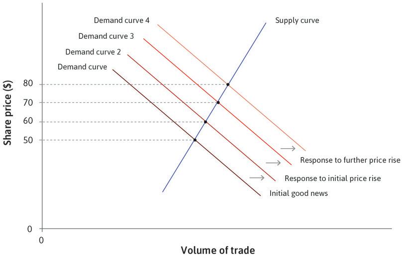
where $a,\ b,\ c,\ d,\ s$ are constants of which $b$, $d$, and $s$ (the speculation parameter) are positive. A supply-and-demand diagram, like Figure 11.15 in the text (reproduced below as Figure 1), then plots different demand curves for each value of $E_t$; an increase in $E_t$ shifts the demand curve to the right.

Suppose the market clears each week: $Q_t^D = Q_t^S$ for all $t$. Then the price in week $t$ is determined by the market-clearing equation:

$$a-bP_t + sE_t = c+dP_t$$

for all $t$, and we can solve for $P_t$ in terms of $E_t$:

$$P_t = \overline{P} + \frac{s}{b+d} E_t, \, \text{ where }\overline{P} = \frac{a-c}{b+d}$$

fundamental value of a share

The share price based on anticipated future earnings and the level of systematic risk, which can be interpreted as a measure of the benefit today of holding the asset now and in the future.

Notice that $\overline{P}$ is what the price would be each week if it were not expected to change. We can think of $\overline{P}$ as the fundamental value of a share.

To discover what happens to the price over time, we have to make some assumptions about market expectations. Let us see what happens if expectations are as accurate as possible from week $1$ onward: that is, market participants are able to forecast price changes correctly. Then

$$E_t = P_{t+1} - P_t$$

for $t=1,\ 2, \ldots \,$ and so on. Substituting this expression for $E_t$ into the preceding equation, we see that:

$$(b+d)(P_t - \overline{P}) = s(P_{t+1} - P_t)$$

Rearranging,

$$P_{t+1} - \overline{P} = R(P_t - \overline{P}), \, \text{ where }R= \frac{b+d+s}{s}\gt1$$

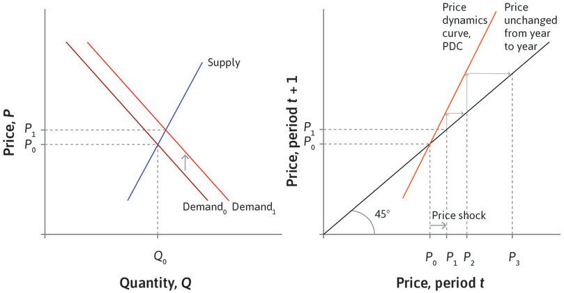
This is the price dynamics curve (PDC) that we discussed in the text. It describes how the price evolves over time. If we begin in period 0 with the price equal to the fundamental value, $P_0 = \overline{P}$, and no shocks occur, then the price will remain at $\overline{P}$ in period 1, 2, and all subsequent periods.

However, since $R \gt 1$ (which follows from the assumptions that demand curves slope downward ($b \gt 0$), supply curves slope upward ($d \gt 0$), and speculation exists ($s \gt 0$), together with our model for expectations), this equilibrium is unstable.

If a shock occurs, temporarily changing the price in period 1 to $P_1 \gt \overline{P}$, then the price will rise again in period 2: the PDC tells us that $P_2$ will be further from the fundamental value than $P_1$. In the next period it will be higher still.

This is the situation illustrated in Figure 11.18 of the main text, reproduced as Figure 2 below. In the diagram, the market is in equilibrium in period 0 ($P_0 = \overline{P}$). The PDC, showing the relationship between $P_t$ and $P_{t+1}$, is represented in the right-hand panel. The PDC cuts the 45$^\circ$ line at $P_0.$ Since $R \gt 1$ the PDC is steeper than 45$^\circ$ line, and after a shock moves the market away from the equilibrium in period 1, the price rises further in every period.

You can see in Figure 2 that not only does the price move further from the equilibrium, it does so at an increasing rate. That is, the price change in each period is bigger than the price change in the last period. To show that our mathematical model predicts this, we can rearrange the equation above to obtain:

$$P_{t+1} - P_t=\frac{b+d}{s}(P_t-\overline{P})$$

and hence also

$$P_{t+2} - P_{t+1}=\frac{b+d}{s}(P_{t+1}-\overline{P})$$

It follows from $P_{t} = \overset{\overline{}}{P} - \frac{s}{b + d}E_{t}$ , $E_{t} = P_{t + 1} - P_{t}$ and the equation above that

$$\frac{P_{t+2} - P_{t+1}}{P_{t+1} - P_{t}}=\frac{P_{t+1}-\overline{P}}{ P_{t}-\overline{P}}=R$$

Again since $R \gt 1$, we can deduce that the price change gets larger each period: that is, the price grows at an increasing rate.

This is the classic example of a bubble: the price rises without bound because it is expected to rise, and will do so for as long as expectations are correct. Similarly, if $P_1\lt\overline{P}$, the price falls continually by increasing amounts. In this case the model predicts that the price will eventually becoming negative, which does not happen in general. It is possible, however, to construct non-linear versions of this model in which the price remains positive forever, becoming smaller and smaller but never hitting zero.

For many asset markets, the supply function above is too simple to be sensible. For example, one may think of the demand for housing as depending on the price of houses and its expected rate of change (these, together with the interest rate, determine the cost of rented accommodation), while the supply of new houses depends on the current price. Let $Q_t$ represent the housing stock in week $t$. Then the supply function above must be replaced by something like:

$$Q_t^S=c+dP_t +(1 - \delta) Q_{t-1}$$

where $\delta$ is the rate of depreciation ($0\lt \delta \lt1$). The mathematics then becomes far more complicated, but the conclusion turns out to be essentially the same. For each value of $Q_0$, there is exactly one initial price, say $F(Q_0)$, with the property that if $P_1= F(Q_0)$ then $P_t$ remains within bounds for all $t\gt1$. Otherwise, $P_t$ explodes or collapses.

Read more: Section 5.1 of Malcolm Pemberton and Nicholas Rau. 2015. Mathematics for economists: An introductory textbook, 4th ed. Manchester: Manchester University Press.