Leibniz

22.2.2 How the monopolist sets the rent-maximizing level of taxes

In our model of tax setting by a dictator who is a political monopolist, the dictator wishes to maximize the political rents that he will receive while in office. But in setting the level of taxes he is constrained by the duration curve: the higher the level of taxes in each year, the fewer additional years he can expect to remain in office. Here we solve the dictator’s constrained optimization problem mathematically, to find his optimal level of tax.

In Leibniz 22.2.1 we derived an expression for the duration curve for a dictator who may be dismissed from office for performance reasons (setting too high a level of taxation) or for reasons unrelated to performance. His expected duration in office, $D$, decreases as the tax in each year, $T$, increases, so we can say that duration is a decreasing function of tax, which we write here as $D=f(T)$.

The dictator’s rent, $R$, depends on both $D$ and $T$. The cost of providing the public services is $C$, so the annual political rent is $T - C$, and the expected total rent obtained by a dictator with expected duration $D$ is:

$$R(D,\ T)=(T-C)D$$

The dictator’s constrained optimization problem is:

$$\text{maximize }(T-C)D \text{ subject to }D=f(T)$$

To solve this problem, we use the constraint to substitute for $D$, so that the rent is $(T-C)f(T)$, and then differentiate with respect to $T$ to obtain the first order condition:

$$f(T)+f'(T)(T-C)=0$$

The first term is the marginal benefit of raising the tax by one unit. The dictator gets an extra unit of rent for the duration $f(T)$ of his or her period in power. The second term is negative because $f(T)$ is a decreasing function. It represents the marginal cost for the dictator of raising the rent, which is that the rent $T-C$ will be received for a shorter period.

The dictator’s optimal tax level $T^*$ satisfies this equation. Once we have found $T^*$, we can determine the corresponding duration from the equation $D^*=f(T^*)$. We will demonstrate this for a particular example below.

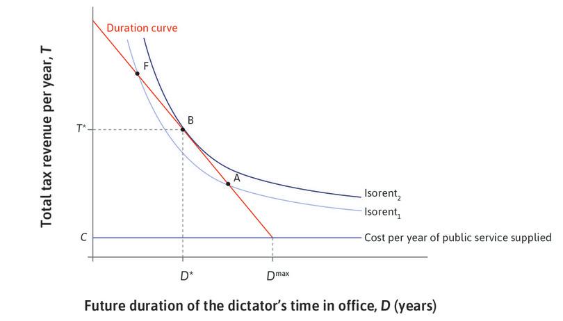
Figure 22.6 from the text, reproduced as Figure 1 below, illustrates the solution of the dictator’s optimization problem.

The solution $(D^*,\ T^*)$ is found at the point B in the diagram, where the duration curve is tangential to an isorent curve. To show that this point is the one we found mathematically above, we can rearrange the first order condition to write it as:

$$-\frac{1}{f'(T)}=\frac{T-C}{D}$$

In this form, the first order condition tells us the same thing as the diagram: at B, the slope of the duration curve is equal to the slope of the isorent curve. To see this, we can calculate the two slopes:

• We have expressed the duration curve as $D^*=f(T^*)$, from which it follows that $dD/dT=f'(T)$. But in the figure we have drawn the curve with $T$ on the vertical axis, so the slope is $dT/dD= 1/f'(T)$. Since $f'(T)$ is negative for all $T$, the left-hand side of the equation above is the absolute value of the slope of the duration curve. We can interpret it as the marginal rate of transformation (MRT) between taxation and duration.

• The equation of an isorent curve is $R(D,\ T)=k$, where $k$ is a constant. To calculate the slope, we could apply the method used for indifference curves in Leibniz 3.2.1. But in this case it is easier to write the isorent curve as $T=C+k/D$, then differentiate to obtain $dT/dD=-k/D^2=-(T-C)/D$. So the right-hand side of the equation above is the absolute value of the slope of the isorent curve, which can be interpreted as the dictator’s marginal rate of substitution (MRS) between taxation and duration.

An example

In the analysis above we did not specify a particular form for the duration curve. But suppose it is linear, as shown in Figure 1. Its equation can then be written $D=f(T)$, where

$$f(T)=D^\text{max}-\frac{1}{s}(T-C)$$

and $s$ is a positive constant. By differentiating $f$ you can verify that $s=-1/f'(T)$, so $s$ represents the absolute value of the slope of the line in Figure 1 (that is, the MRT). With this duration curve the first order condition $f(T)+f'(T)(T-C)=0$ becomes:

$$D^\text{max}-\frac{1}{s}(T-C) -\frac{1}{s}(T-C)=0$$

which can be solved to obtain:

$$T^*=C+\frac{s}{2} D^\text{max}$$

and, since $D^*=f(T^*)$:

$$D^*= \frac{1}{2} D^\text{max}$$

Notice that the level of taxation chosen by the dictator will be higher when the duration curve is steeper (that is, when $s$ is larger). This is similar to the case of a profit-maximizing firm, which sets a higher price when the demand curve is less elastic (steeper). In this case, however, the corresponding expected duration will be the same whatever the slope $s$ of the duration curve. We will return to this point in Leibniz 22.3.1.