Leibniz

5.7.1 Angela’s choice of working hours when she pays rent

In Leibniz 5.4.2 we solved Angela’s constrained optimization problem for the decisions she made as an independent farmer. Now we look at the case in which Bruno owns the land, and Angela has to pay rent in order to produce grain. We will see that Angela’s quasi-linear preferences have an important implication for the effect of the rent on her decision.

As before, Angela’s preferences are represented by a quasi-linear utility function:

$$U(t,\ c) = v(t) + c$$

where $t$ represents her daily hours of free time and $c$ the number of bushels of grain she consumes per day. The function $v$ is increasing and concave. Her feasible frontier shows how the number of bushels of grain she can consume per day, $y$, depends on the free time she takes.

When Angela was an independent farmer, she could consume all the grain she produced. Her feasible frontier was $c=g(t)$, where $g'(t)\lt0$ and $g''(t)\lt0$, and her constrained optimization problem was to choose $t$ and $c$ to maximize $v(t) + c$, subject to the constraint $c =g(t)$, giving us the first-order condition:

$$v'(t) + g'(t)=0$$

Her optimal choice of free time, $t^*$, is the value of $t$ that satisfies this equation. Remember that her MRS is $v'(t)$ and her MRT is $-g'(t)$; the optimal choice is where MRS = MRT.

How does the problem change when Angela pays rent?

Suppose she has to pay $c_0$ bushels of grain per day to her landlord Bruno for the right to operate her farm. This means that Angela’s consumption of grain is less than her production. If she takes $t$ hours of free time she produces $g(t)$ bushels of grain as before, but now her consumption will be:

$$c= g(t) -c_0$$

In this case, her constrained optimization problem is to choose $t$ and $c$ to maximize $v(t) + c$, subject to the constraint $c =g(t)-c_0.$

But the first-order condition for her optimal choice of free time is exactly the same as before:

$$v'(t) + g'(t)=0$$

so she will choose exactly the same amount of free time $t^*$ as she did in the case when she did not have to pay rent. Of course, this means that she will produce the same amount of grain as before, although her consumption will be lower by the amount of rent she has to pay.

Why does this happen? When Angela has to pay rent, she takes $t$ hours of free time and pays $c_0$ to Bruno, so her consumption will be lower. But the rate at which she can transform free time into consumption for herself doesn’t change. An additional hour of work will give her just as much additional grain as when she didn’t have to pay rent, so her MRT is still $g'(t)$. And the lower consumption doesn’t affect her marginal rate of substitution either, because of her quasi-linear preferences: her MRS is $v'(t)$ irrespective of her consumption of grain.

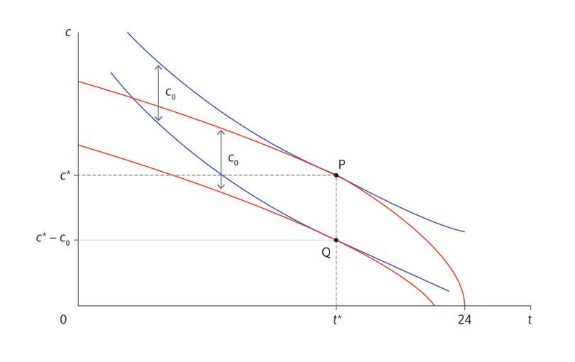
The effect of payment of rent is shown in Figure 1. Angela’s original feasible frontier as an independent farmer, $c=g(t)$, is the upper red curve. Her optimal choice of free time and consumption in that case is at P. When she pays a rent of $c_0$, her feasible frontier for consumption and free time is shifted vertically downward by $c_0$ units. This is the lower red curve in the diagram: $c=g(t)-c_0$.

Angela’s new optimal point is Q: she continues to have $t^*$ hours of free time per day, and her daily consumption of grain is now $c^* - c_0$ bushels. You can see the effect of quasi-linearity in the figure: quasi-linear indifference curves have the same slope as you move up or down a vertical line.

We have shown that Angela will choose the same amount of free time whatever the level of the rent $c_0$. She makes the same choice if the rent is zero—the independent farmer case—and she would still make the same choice if $c_0$ were negative: for example, if she had no landlord and received a subsidy from the government for working on her farm.

The result that payment of rent does not change Angela’s allocation of time means that any distributional conflict between her and Bruno concerns only how much grain each of them gets to consume. Because of her quasi-linear preferences, Angela’s hours of work are determined independently of how the grain is distributed, so the size of the pie and how it is divided are entirely separate issues. The assumption of quasi-linearity is made in Unit 5 to enable us to think about these two issues separately.

Read more: Sections 17.1 to 17.3 of Malcolm Pemberton and Nicholas Rau. 2015. Mathematics for economists: An introductory textbook, 4th ed. Manchester: Manchester University Press.