Leibniz

7.6.1 Marginal revenue and marginal cost

One way to determine the price and quantity that maximize the profits of a firm such as Beautiful Cars is to find the point where the demand curve is tangent to an isoprofit curve. This Leibniz introduces an alternative method using the firm’s marginal revenue and marginal cost.

Remember that Beautiful Cars’ profit, $\Pi$, is equal to its total revenue from selling cars, minus its total cost of producing them:

$$\Pi = PQ - C(Q)$$

The inverse demand curve, $P=f(Q)$, tells us the maximum price $P$ at which $Q$ cars can be sold, so we can write revenue as a function of $Q$ alone, which we call the revenue function and denote by $R(Q)$. Thus:

$$R(Q) = f(Q) \times Q$$

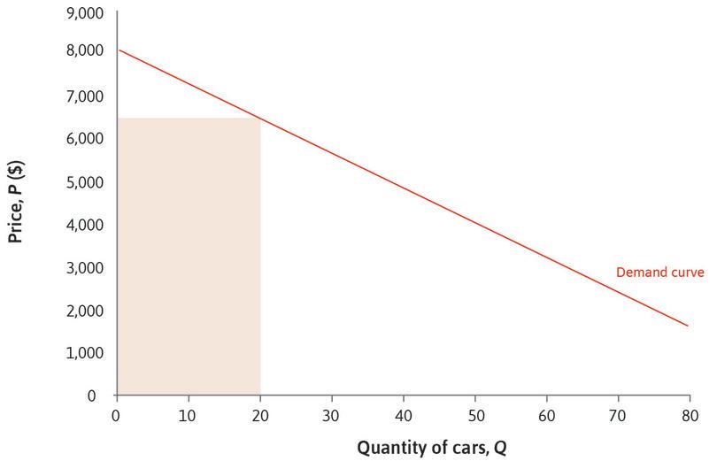
Revenue at any point on the demand curve can be represented graphically as the red rectangle below the curve, as shown in Figure 7.12a of the text, reproduced as Figure 1.

The expression for profits, above, can be written as a function of output $Q$, as the difference between the total revenue function $R(Q)$ and total cost $C(Q)$:

$$\Pi = R(Q) - C(Q)$$

To find the value of $Q$ that maximizes profit, we differentiate with respect to $Q$, to obtain the first-order condition $d\Pi/dQ =0$, which implies that:

$$R'(Q) = C'(Q)$$

marginal cost

The effect on total cost of producing one additional unit of output. It corresponds to the slope of the total cost function at each point.

marginal revenue

The increase in revenue obtained by increasing the quantity from Q to Q + 1.

The term $C'(Q)$ on the right-hand side of the equation is the firm’s marginal cost (MC)—the rate at which cost increases as output rises. Similarly, $R'(Q),$ the derivative of the revenue function, is the rate at which revenue rises with output, and it is known as marginal revenue (MR). Thus, the first-order condition for profit maximization may be written as:

$$\text{MR}=\text{MC}$$

So the first-order condition tells us that, when $Q$ is at its profit-maximizing level, the marginal revenue is equal to the marginal cost.

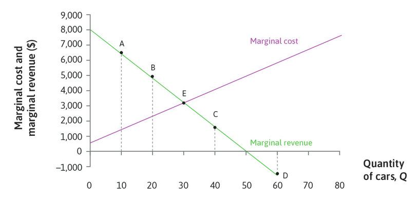
The marginal cost curve (that is, the function $C'(Q)$) shows how marginal cost changes as output changes. In the case of Beautiful Cars, we know that marginal cost increases with output, so the MC curve is upward-sloping. Similarly, the function $R'(Q)$ is the marginal revenue curve, showing how marginal revenue changes with output. In the text we drew the MR curve as downward-sloping. Figure 1 reproduces the middle panel of Figure 7.12b from the text, showing both curves.

The profit-maximizing quantity lies at the point where the two curves cross—at point E in Figure 2, where $R'(Q=C'(Q)$. Since Beautiful Cars has an upward-sloping MC and downward-sloping MR, there is just one point of intersection.

At point E, the company produces 32 cars. As explained in the interactive for Figure 7.12b in the text, we can see that this is profit-maximizing by noting that the marginal cost of producing more than 32 cars would be greater than the marginal revenue generated (MC > MR), while the opposite would be true if fewer than 32 were produced.

But note that if the curves had sloped differently this argument might not have worked. If MC sloped downward (which can happen, if the firm has economies of scale) and MR sloped upward (which would be unusual, but can happen for some demand functions), the point of intersection would be a profit-minimizing point (try drawing the curves and explaining to yourself why this must be true).

In general, if we can find a solution $Q^*$ to the first-order condition MC = MR, we can say that it is the profit-maximizing quantity if MC < MR when $Q\lt Q^*$ and MC > MR when $Q\gt Q^*$.

The relationship between the two methods

We now show that the first-order condition for profit maximization derived above, $\text{MR}=\text{MC}$, is equivalent to the first-order condition for profit maximization given in Leibniz 7.5.1. Using the rule for differentiating a product to differentiate $R(Q) = Qf(Q)$, we see that:

$$\text{MR} = \frac{d}{dQ} (Qf(Q)) = f(Q) + Qf'(Q) = P+Qf'(Q)$$

Thus the first-order condition $\text{MR} = \text{MC}$ may be written:

$$P+Qf'(Q) = \text{MC}$$

Rearranging,

$$f'(Q)= \frac{ \text{MC} -P}{Q}$$

which is the first-order condition of Leibniz 7.5.1. Remember that it can be interpreted as saying that the slope of the demand curve is equal to the slope of the isoprofit curve.

We drew very different diagrams to illustrate the two forms of the first-order condition. MC = MR is illustrated by drawing the MC and MR curves and finding the intersection. The other form can be illustrated by drawing the demand and isoprofit curves, and showing the tangency point.

This MC = MR method is often useful in the analysis of firms’ behaviour. In empirical work it is sometimes easier to estimate a revenue function than a demand function. In Leibniz 7.8.1, when we introduce the concept of the elasticity of demand, we shall see yet another useful way of writing the first-order condition. But whichever method is used, the first-order conditions are equivalent, and the solution for the profit-maximizing quantity is therefore the same.

Read more: Sections 6.4 and 8.1 of Malcolm Pemberton and Nicholas Rau. 2015. Mathematics for economists: An introductory textbook, 4th ed. Manchester: Manchester University Press.