Unit 16 Technological progress, employment, and living standards in the long run
Themes and capstone units
How long-term trends and differences in living standards and unemployment between countries are the result of technological progress, institutions, and policies
- The increasing use of machinery and other capital goods in production, along with technological progress made possible by increasing knowledge, have been the foundation for rising living standards in the long run.
- The ‘creative destruction’ of older ways of producing goods and organizing production has led to continuous job loss as well as job creation, but not higher unemployment in the long run.
- A country’s economic institutions and policies can be evaluated by their capacity to keep involuntary unemployment low and to sustain increases in real wages.
- Many successful economies have provided extensive forms of co-insurance against the job losses arising from both creative destruction and competition from other economies, so that most citizens of these nations welcome both technological change and the global exchange of goods and services.
- The main difference between high-performing economies and laggards is that the institutions and policies of high performers incentivize their main actors to increase the size of the pie, rather than fighting over the size of their slice.
In 1412, the city council of Cologne prohibited the production of a spinning wheel by a local craftsman because it feared unemployment among textile manufacturers that used the hand spindle. In the sixteenth century, new ribbon-weaving machines were banned in large parts of Europe. In 1811, in the early stage of the Industrial Revolution in England, the Luddite movement protested forcefully against new labour-saving machinery, such as spinning machines that allowed one worker to produce the amount of yarn previously produced by 200 workers. The movement was led by a young unskilled artisan, Ned Ludd, who allegedly destroyed the spinning machines.1
The Swiss economist Jean-Charles-Léonard de Sismondi (1773–1842) contemplated a new world ‘where the King sits alone on his island, endlessly turning cranks to produce, with automatons, all that England now manufactures’. The increasing use of information technology has caused contemporary economists, including Jeremy Rifkin, to voice the same fears.2
Sismondi and Rifkin made plausible arguments. But as we saw in Unit 1, as a result of labour-saving innovations, many countries moved to the upward part of the hockey stick and experienced sustained growth in living standards. Workers were paid more–remember the real wage hockey stick from Unit 2 (Figure 2.1). The ‘end of work’ also hasn’t happened yet, though in 1935 Bertrand Russell, a philosopher, expressed anticipation rather than fear of the end of work, arguing that: ‘[T]here is far too much work done in the world, that immense harm is caused by the belief that work is virtuous, and that what needs to be preached in modern industrial countries is quite different from what always has been preached.’
Technological progress has not created rising unemployment rates. Instead it has raised the lowest wage that firms can pay while still covering their costs. As a result, technological progress expands the resources the firm has to invest in increasing production, and it also incentivizes continued investment. By focusing only on the destruction of jobs, those who worry about the end of work have ignored the fact that labour-saving technological progress also induces the investment that helps to create jobs.
In most economies for which data is available, at least 10% of jobs are destroyed every year, and about the same number of new ones are created. In France or the UK, every 14 seconds a job is destroyed and another one created. This is part of the creative destruction process at the heart of capitalist economies that we described in Units 1 and 2.
Those who lose their jobs bear substantial costs in the short run. The short run may not seem very short to them: it can last years or even decades. Those who benefit may be the children of the handloom weaver displaced by the power loom, or the children of the unemployed typist who was displaced by the computer. They benefit by finding a job in an occupation that is more productive than the job their parents did, and they may share in the benefit from the new goods and services that are available because the power loom or the computer exist.
The destructive part of creative destruction affects occupations that may often be concentrated in particular regions, with large losses in wages and jobs. Families and communities who are the losers often take generations to recover. Like ‘short run’, the term ‘average’ often hides the costs to the workers displaced and communities destroyed by the introduction of new technologies.
Today, for example, information and communication technology (ICT) is reshaping our societies. ICT is replacing much of routine labour, in many cases further impoverishing the already poor. People who would have previously anticipated rising living standards have fewer job opportunities.
Nevertheless, most people benefit from the fall in prices due to the new technology. For better or worse, creative destruction as a result of technological progress is part of the dynamism of the capitalist economic system. And while lives have been disrupted and the environment increasingly threatened by this dynamism, the introduction of improved technologies is also the key to rising living standards in the long run. We shall see that:
- technological change is constantly putting people out of work
- but the countries that have avoided high levels of unemployment are among those in which the productivity of labour has increased the most
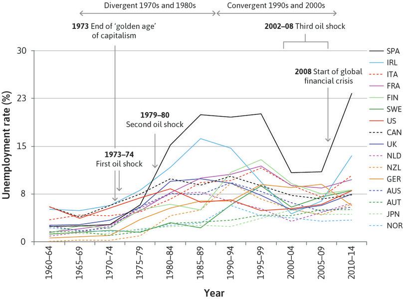
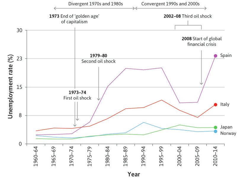
Figure 16.1 shows unemployment rates for 16 OECD countries from 1960 to 2014.
Unemployment rates in selected OECD countries (1960–2014).
Figure 16.1 Unemployment rates in selected OECD countries (1960–2014).
Data from 1960–2004: David R Howell, Dean Baker, Andrew Glyn, and John Schmitt. 2007. ‘Are Protective Labor Market Institutions at the Root of Unemployment? A Critical Review of the Evidence’. Capitalism and Society 2 (1) (January). Data from 2005 to 2012: OECD. 2015. OECD Statistics.
Unemployment rates were low and quite similar in the 1960s, and then diverged in the 1970s, reflecting in part the different responses to the oil shocks described in Unit 14. Of these countries, only Japan (JPN), Austria (AUT), and Norway (NOR) had unemployment rates that stayed below 6% over the entire period. In Spain (SPA), unemployment was around 20% from the mid 1980s to the end of the 1990s. It then halved in the 2000s before jumping back above 20% following the financial crisis and Eurozone crisis from 2009. In this respect Germany (GER) is unusual: unemployment fell in the years following the global financial crisis.
While there has been no upward trend in unemployment rates over the long run, there have been two important developments in the labour market that have accompanied the growth in living standards. As we saw in Unit 3 (Figure 3.1), average annual hours worked by people with jobs have fallen. In addition, a larger fraction of adults are working for pay, which is mainly due to the rise in the proportion of women who do paid work.
The patterns of unemployment in Figure 16.1 are not explained by national differences in the rate of innovation, or waves of innovation over time. They reflect differences in the institutions and policies in force in the countries.
As production has become more capital-intensive, how have living standards improved over the long run without producing mass unemployment? We begin by studying the accumulation of capital (the increasing stock of machinery and equipment) and infrastructure (such as roads and ports), which have always been fundamental to the dynamism of capitalism.
Exercise 16.1 Wealth and life satisfaction
As we saw in Unit 3, technological progress increases your hourly productivity. This means that by working the same number of hours you could thus produce and consume more, or you can produce and consume the same amount of goods while working fewer hours and enjoying more free time.
The economist Oliver Blanchard argues that the difference in output per capita between the US and France is partially due to the fact that relative to those in the US, the French have used some of the increase in productivity to enjoy more free time rather than raise consumption.
- Think about two countries, one that has lower GDP per capita due to fewer hours worked, and another that has higher GDP per capita due to more hours worked (such as France and the US). Assuming that overall life satisfaction consists only of free time and consumption, in which country would you expect overall life satisfaction to be higher, and why? Clearly state any assumptions you make about the preferences of residents in each country.
- Considering only working hours and GDP per capita, which country (France or the US) would you prefer to live in, and why? How would your answer change if you considered other factors as well?
Question 16.1 Choose the correct answer(s)
Figure 16.1 is a graph of unemployment rates for 16 OECD countries from 1960 to 2014.
Based on this information, which of the following statements is correct?
- Most countries had lower unemployment rates in the 1960s than in the 1980s and 1990s, and most saw some decline in the late 1990s, suggesting a mild positive correlation.
- The graphs show no clear upward trend in unemployment since the 1980s.
- While most countries had higher unemployment after the oil shocks than before, some saw very large increases, like Ireland and Spain, while others saw small increases, like Japan, Austria, and Norway.
- The unemployment rate actually fell in Germany after 2008.
16.1 Technological progress and living standards
- innovation rents
- Profits in excess of the opportunity cost of capital that an innovator gets by introducing a new technology, organizational form, or marketing strategy. Also known as: Schumpeterian rents.
- creative destruction
- Joseph Schumpeter’s name for the process by which old technologies and the firms that do not adapt are swept away by the new, because they cannot compete in the market. In his view, the failure of unprofitable firms is creative because it releases labour and capital goods for use in new combinations.
- capital goods
- The equipment, buildings, raw materials, and other inputs used in producing goods and services, including where applicable any patents or other intellectual property that is used.
In Unit 2 we saw how firms could earn Schumpeterian innovation rents by introducing new technology. Firms that fail to innovate (or copy other innovators) are unable to sell their product for a price above the cost of production, and eventually fail. This process of creative destruction led to sustained increases in living standards on average because technological progress and the accumulation of capital goods are complementary: each provides the conditions necessary for the other to proceed.
- New technologies require new machines: The accumulation of capital goods is a necessary condition for the advance of technology, as we saw in the case of the spinning jenny.
- Technological advance is required to sustain the process of capital goods accumulation: It means that the introduction of increasingly capital-intensive methods of production continues to be profitable.
The second point here needs explanation. Start with the production function that we used in Units 2 and 3. We discovered that output depends on labour input, and that the function describing this relationship shifts upward with technological progress, so that the same amount of labour now produces more output. In Unit 3 the farmer had a fixed amount of land: we assumed the amount of capital goods was fixed. But as we have seen, the amount of capital goods which the modern worker uses is vastly greater than that used by farmers in the past.
- capital-intensive
- Making greater use of capital goods (for example machinery and equipment) as compared with labour and other inputs. See also: labour-intensive.
- labour productivity
- Total output divided by the number of hours or some other measure of labour input.
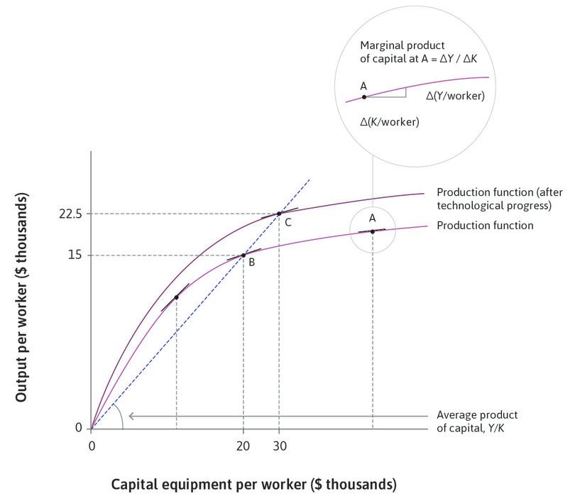
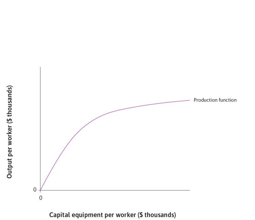
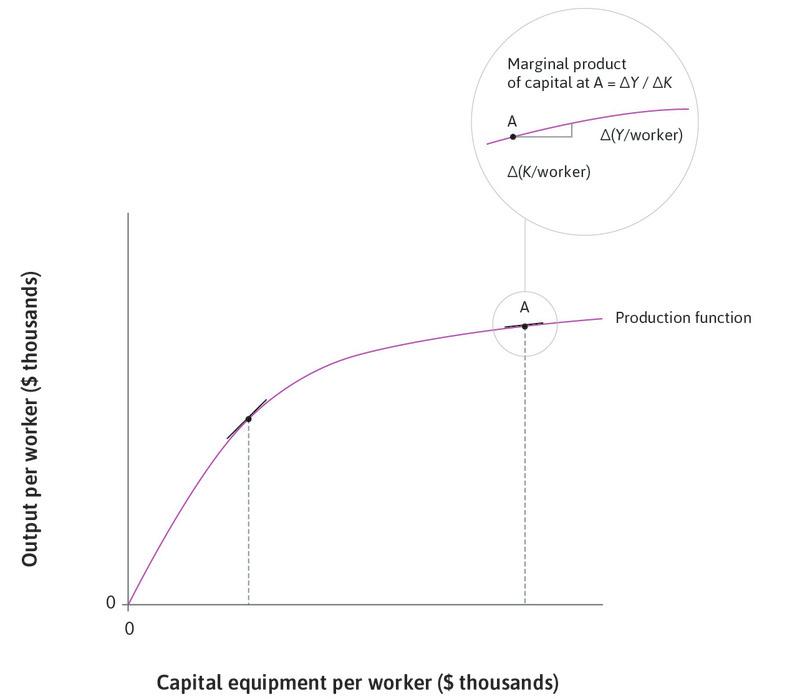
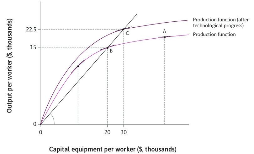
Now we include capital goods (machinery, equipment, and structures) explicitly in the production function. If you look at the horizontal axis in Figure 16.2, you will see that it records the amount of capital goods per worker. This is a measure of what is called the capital intensity of production. On the vertical axis, we have the amount of output per worker, also known as labour productivity.
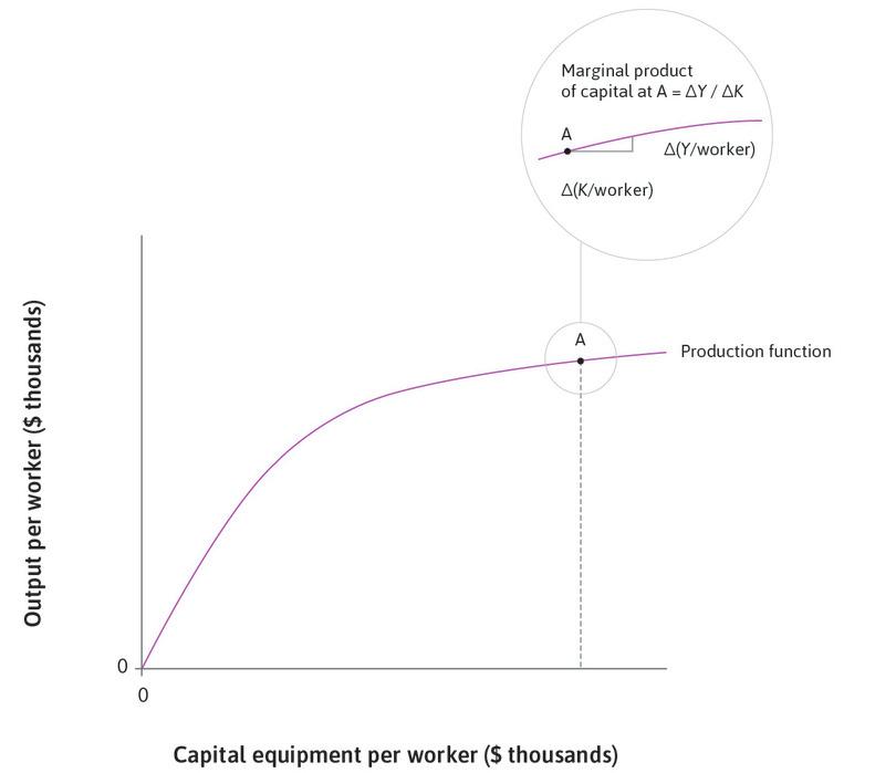
As was the case in Unit 3, the production function describes diminishing marginal returns: as the worker works with more capital goods, output increases, but at a diminishing rate (Charlie Chaplin showed in the 1936 film Modern Times that there is a limit to the number of machines a worker can make use of). This means that with increasing quantities of capital goods, we have a diminishing marginal product of capital goods. The slope of the production function at each level of capital per worker shows the marginal product of capital. It shows how much output increases if capital equipment per worker increases by one unit.
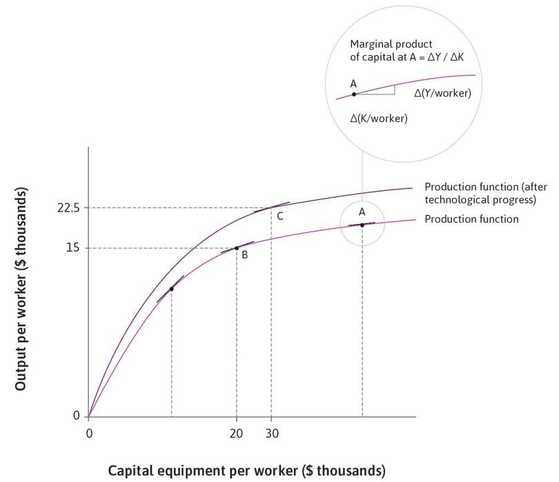
The magnified section at point A in Figure 16.2 shows how the marginal product of capital is calculated: note that Y/worker is used as shorthand for output per worker, and the marginal product of capital (MPK) is ΔY/ΔK. The marginal product of capital at each level of capital per worker is the slope of the tangent to the production function at that point.
Leibniz: Malthusian economics
Leibniz: Labour and production
Previous Leibnizes have showed how to use calculus to calculate the MPK at any point on a given production function. Take a moment to have another look at them.
- concave function
- A function of two variables for which the line segment between any two points on the function lies entirely below the curve representing the function (the function is convex when the line segment lies above the function).
We can see from Figure 16.2 that the marginal product of capital is falling as we move along the production function. A production function that exhibits diminishing returns to capital is concave. Concavity captures the fact that output per worker increases with capital per worker, but less than proportionally.
Concavity means that an economy will not be able to sustain growth in output per worker simply by adding more of the same type of capital. At a certain point, the marginal productivity of capital becomes so low that it is not worth investing any further. As we saw in Unit 14, business owners will invest domestically only if the return is higher than the return to buying bonds (the yield) or investing abroad, and at the same time, high enough that they do not simply want to spend their profits on consumption goods.
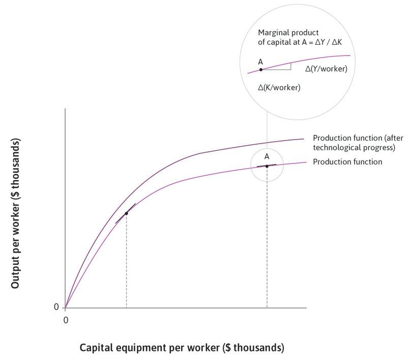
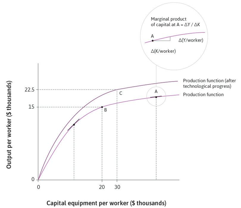
Sustained economic growth requires technological change that increases the marginal productivity of capital. This rotates the production function upwards and makes it profitable to invest domestically, leading to increased capital intensity. Follow the steps in the analysis in Figure 16.2 to see how the combination of technological change and capital investment raises output per worker.
- Taylorism
- Innovation in management that seeks to reduce labour costs, for example by dividing skilled jobs into separate less-skilled tasks so as to lower wages.
New technology can also refer to new ways of organizing work. Remember that a technology is a set of instructions for combining inputs to make output. The managerial revolution in the early twentieth century called Taylorism is a good example: labour and capital equipment were reorganized in a streamlined way, and new systems of supervision were introduced to make workers work harder. More recently, the information technology revolution allows one engineer to be connected with thousands of other engineers and machines all over the world. The ICT revolution therefore rotates the production function upward, increasing its slope at every level of capital per worker.
In Figure 16.2, you can see a dotted blue line from the origin through the production functions for the old and new technologies. The slope of this line tells us the amount of output per unit of capital goods at the point where it intersects the production function: it is the amount of output per worker divided by the capital goods per worker. From the diagram, we note that points B and C on the two production functions have the same output per unit of capital goods.
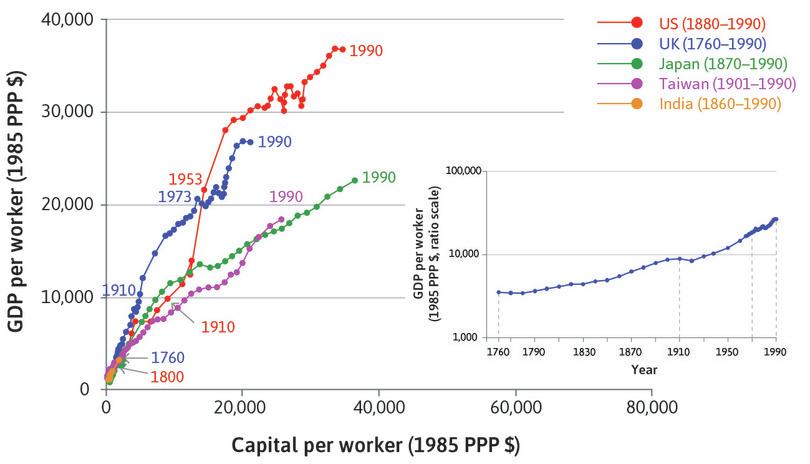
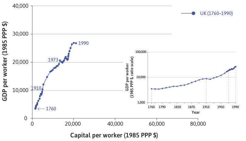
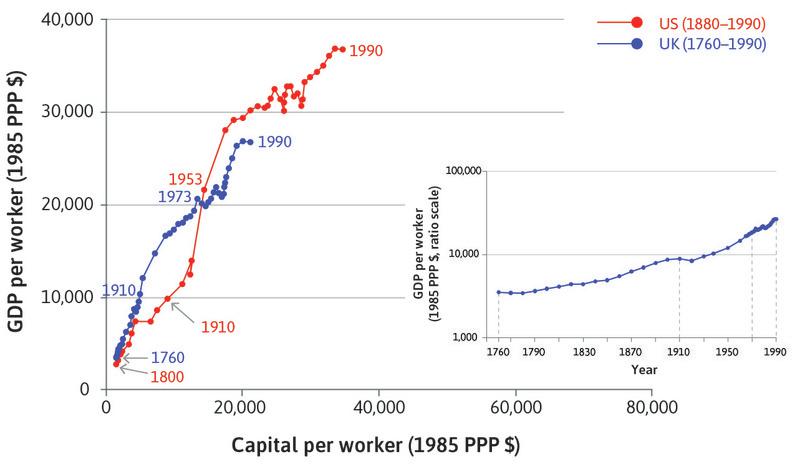
To see how technological progress and capital accumulation shaped the world, we focus on the countries that have been the technology leaders. Britain was the technological leader from the Industrial Revolution until the eve of the First World War, when the US took over leadership. Figure 16.3 has capital per worker on the horizontal axis and output per worker on the vertical axis.
We can now look at the path traced out over time by the UK and the US. Looking first at Britain, the data begins in 1760 (the bottom corner of the chart) and ends in 1990 with much higher capital intensity and productivity. The bottom right-hand side of the diagram shows the same points in the familiar hockey-stick chart for GDP per worker. As Britain moved up the hockey stick over time, both capital intensity and productivity rose. In the US, productivity overtook the UK by 1910 and has remained higher since. In 1990, the US had higher productivity and capital intensity than the UK.
Figure 16.3 shows that the countries that are rich today have seen labour productivity rise over time as they became more capital-intensive. For example, if we look at the US, capital per worker (measured in 1985 US dollars) rose from $4,325 in 1880 to $14,407 in 1953, and $34,705 in 1990. Alongside this increase in capital intensity, US labour productivity rose from $7,400 in 1880 to $21,610 in 1953, to $36,771 in 1990. John Habakkuk, an economic historian, has argued that wages were high for factory workers in the US in the late nineteenth century because they had the option to move to the west of the country: therefore the factory owners had the incentive to develop labour-saving technology.3
Productivity growth has reduced labour input per unit of output: the fear of the Luddites and the forecasts of the ‘end of work’ authors was that this would cause permanent job loss.
From Figure 16.3 it is clear that the historical paths traced out by these economies are not curved like the single production function in Figure 16.2. This is because they experienced a combination of capital accumulation and technological progress. Successfully growing economies move along paths similar to the blue dotted line between B and C in Figure 16.2.
We know from Unit 1 that other countries moved up the hockey stick at very different times. Consider Japan, Taiwan and India in Figure 16.3. Notice that by 1990, capital per worker in Japan was not only higher than in the US, but also almost twice as high as in Britain. Japan had reached this level in less than half the time it took Britain. Taiwan in 1990 was also more capital-intensive than Britain. The lead in mass production and science-based industries that the US had established was eroded as other countries invested in education and research, and adopted American management techniques.4
Interpreting Figure 16.3 using the model of the production function in Figure 16.2 shows that countries adopted more capital-intensive methods of production as they became richer. However, while Japan and Taiwan both experienced substantial technological progress, the fact that output per worker remained below that of both the US and Britain means that they remained on a lower production function.
To summarize:
- Technological progress shifted the production function up: It was stimulated by the prospect of innovation rents.
- This offset the diminishing marginal returns to capital: Capital productivity, measured by the slope of a ray from the origin, remained roughly constant over time in the technology leaders.
Technological progress played a crucial role in preventing diminishing returns from ending the long-run improvement in living standards resulting from the accumulation of capital goods.
Question 16.2 Choose the correct answer(s)
The following diagram shows an economy’s production function before and after technological progress:
Based on this information, which of the following statements is correct?
- The average product of capital at A is 15,000/20,000 = 0.75.
- The marginal product of capital at A is the slope of the production function at A.
- This means that the slope gets flatter as it moves to the right.
- On the diagram, A and B have the same average product of capital. These are not at the same level of capital per worker, however. At a given level of capital per worker, both average and marginal products of capital rise with technological progress.
16.2 The job creation and destruction process
Labour-saving technological progress of the type illustrated in Figures 16.2 and 16.3 allows more outputs to be produced with a given amount of labour, and it also contributes to the expansion of production. By incentivizing investment, it compensates for some of the jobs it has destroyed, and may even create more jobs than previously existed. When more jobs are created than destroyed in a given year, employment increases. When more jobs are destroyed than created, employment decreases.
- stock
- A quantity measured at a point in time. It’s units do not depend on time. See also: flow.
- flow
- A quantity measured per unit of time, such as annual income or hourly wage.
We know that at any moment there are some people who are involuntarily unemployed. They would prefer to be working, but don’t have a job. The number of unemployed people is a stock variable, measured without a time dimension. It changes from day to day, or year to year, as some of the jobless are hired (or give up seeking work), other people lose a job, and yet others decide to seek work for the first time (young people leaving school or university, for example). Those without work are sometimes called the ‘pool’ of the unemployed: people getting a job or ceasing to look for one exit the pool, while those who lose their jobs enter the pool. The number of people getting and losing jobs is a flow variable.
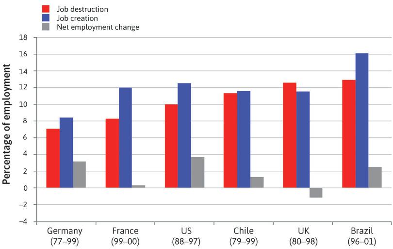
The total job reallocation process is the sum of job creation and destruction. Compared to that, the net growth of employment is typically small and positive.
Figure 16.4 shows the job destruction, job creation, and net employment growth in some countries. Note that in the UK from 1980 to 1998, more jobs were destroyed than created: net employment growth was negative. Across a set of countries at different stages of development, and with different openness to international trade, we see a fairly similar rate of job reallocation. In most countries, about one-fifth of jobs are created or destroyed each year, in spite of widely varying rates of net employment growth.
Job destruction, job creation, and net employment across countries.
Figure 16.4 Job destruction, job creation, and net employment across countries.
John Haltiwanger, Stefano Scarpetta, and Helena Schweiger. 2014. ‘Cross Country Differences in Job Reallocation: The Role of Industry, Firm Size and Regulations’. Labour Economics (26): pp. 11–25.
Now imagine an economic system in which new jobs are created at a rate of 2% each year, and job destruction is banned (that is, the job destruction rate is zero). This economy would also see a net employment growth of 2%. This is what a planner might seek to do. Figure 16.4 shows this is not the way a capitalist economy works in practice: there is no planner. Competition and the prospect of gaining economic rents both mean that creating some jobs often implies destroying others.
To understand how job creation and destruction take place in an industry, we look at the impact of the information technology revolution in the US retail sector since the 1990s. The adoption of systems that electronically link cash registers to scanners, credit card processing machines, and to management systems for both inventories and customer relationships allowed tremendous increases in output per worker. Think of the volume of retail transactions handled per cashier in a new retail outlet.
Research shows that labour productivity growth in the retail sector was entirely accounted for by more productive new establishments (such as retail units or plants) displacing much less productive existing establishments (including older establishments of the same firm, as well as shops and plants owned by others, where jobs were lost).
We showed the massive expansion of employment in the US firm Walmart in Figure 7.1 of Unit 7. Walmart’s growth was partly based on opening more efficient out-of-town stores, made possible by new retail and wholesale technologies.
For the manufacturing sector, detailed evidence collected from all the firms in the economy shows how productivity growth takes place through the creation and destruction of jobs inside firms, and by their entry and exit. Data for Finland in the years from 1989 to 1994, for example, shows that 58% of productivity growth took place within firms (similar to the Walmart example). The exit of low-productivity firms contributed to a quarter of the increase, and 17% was contributed by the reallocation of jobs and output from low- to high-productivity firms.
The French construction industry provides another example of the reallocation of work from weaker to stronger firms. According to the French National Institute of Statistics, more of the jobs in the economy were destroyed than created in firms with very low productivity (in the bottom 25%). Between 1994 and 1997, these firms created 7.1% of new jobs and destroyed 16.1%, implying that employment in those firms shrank by 9.0%. In contrast, job creation exceeded destruction (17.1% against 11.8%) in the top 25% of construction firms.
Exercise 16.2 Schumpeter revisited
- In Unit 2 we discussed how Joseph Schumpeter characterized capitalist economies by the process of ‘creative destruction’. In your own words, explain what this term means.
- Based on this definition, give examples of destruction and creation, and identify the winners and the losers in the short and long run.
16.3 Job flows, worker flows, and the Beveridge curve
- bargaining power
- The extent of a person’s advantage in securing a larger share of the economic rents made possible by an interaction.
- procyclical
- Tending to move in the same direction as aggregate output and employment over the business cycle. See also: countercyclical.
- countercyclical
- Tending to move in the opposite direction to aggregate output and employment over the business cycle.
- acyclical
- No tendency to move either in the same or opposite direction to aggregate output and employment over the business cycle.
- co-insurance
- A means of pooling savings across households in order for a household to be able to maintain consumption when it experiences a temporary fall in income or the need for greater expenditure.
- Beveridge curve
- The inverse relationship between the unemployment rate and the job vacancy rate (each expressed as a fraction of the labour force). Named after the British economist of the same name.
Jobs are created and destroyed by business owners and managers seeking to gain Schumpeterian innovation rents, and in response to the pressure of competition in markets for goods and services. For most workers this means that nothing is permanent: in the course of a lifetime, people move in and out of many jobs (often not by choice). Sometimes people move from job to job, but they move in and out of unemployment too.
In Unit 5, we looked at the decisions of an employer (Bruno) and an employee (Angela) about her work hours and rent. Once Bruno’s gun was replaced by a legal system and contracts, we saw that taking a job was a voluntary arrangement entered into for mutual gain. The balance of bargaining power may have been unequally distributed but the exchange was, nevertheless, voluntary.
When a worker leaves a job, it may be voluntary, but it can also be an involuntary temporary lay-off (dictated by product demand conditions facing the firm), or a redundancy (the job has been eliminated).
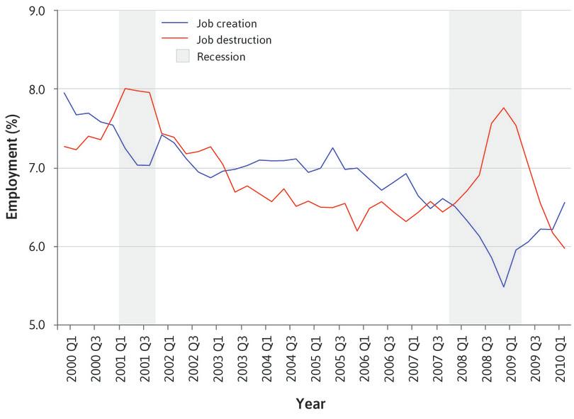
Jobs are also created, as can be seen by the movement of job destruction and creation in the US in Figure 16.5. Job creation is strongly procyclical: this means that it rises in booms, and falls during recessions. Conversely, job destruction is countercyclical: it rises during recessions (if the change in a variable was not correlated with the business cycle, it would be called acyclical). The next section will show how aggregate policies interact with those movements in job flows and worker flows.
This intense job reallocation process and the ability of the government to provide co-insurance led the English economist and politician Lord William Beveridge (1879–1963) to become the founding father of the UK social security system. He is also remembered among economists because, like Bill Phillips, they bestowed on Beveridge one of their highest honours: they named the Beveridge curve after him.
We met the concept of co-insurance in Unit 13, when we explained how households that have been fortunate during a particular period use their savings to help a household hit by bad luck, and in Unit 14, when we explained how correlated risk limits the usefulness of co-insurance, helping to explain the government’s role in providing co-insurance through a system of unemployment benefits.
Job creation and destruction during business cycles in the US (2000 Q1–2010 Q2).
Figure 16.5 Job creation and destruction during business cycles in the US (2000 Q1–2010 Q2).
Steven J. Davis, R. Jason Faberman, and John C Haltiwanger. 2012. ‘Recruiting Intensity During and After the Great Recession: National and Industry Evidence’. American Economic Review 102 (3): pp. 584–588.
The Beveridge curve
Beveridge suggested a simple relationship between job vacancy rates (the number of jobs available for workers) and the level of unemployment (the number of workers looking for jobs), expressed as a fraction of the labour force.
Beveridge noticed that when unemployment was high, the vacancy rate was low; and when unemployment was low, the vacancy rate was high:
- During recessions, there will be high unemployment: When the demand for a firm’s product is declining or growing slowly, firms can manage with their current staff even if a few of them quit or retire. As a result, they advertise fewer positions. In the same conditions of weak demand for firms’ products, people will be laid off or their jobs entirely eliminated.
- During booms, unemployment will decline: The number of vacant jobs posted by firms increases, and more workers will be employed to cope with rising demand for products.
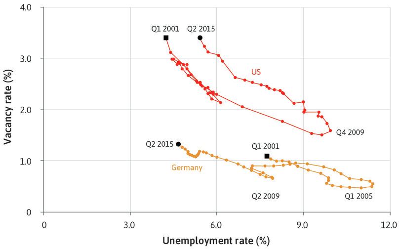
The downward-sloping relationship between the vacancy rate and the unemployment rate over the business cycle is illustrated in Figure 16.6, which shows two examples of what came to be called the Beveridge curve, using data from Germany and the US. Each dot represents a quarter, from 2001 Q1 until 2015 Q2.
Beveridge curves for the US and Germany (2001 Q1–2015 Q2).
Figure 16.6 Beveridge curves for the US and Germany (2001 Q1–2015 Q2).
OECD Employment Outlook and OECD Labour Force Statistics: OECD. 2015. OECD Statistics.
Why are there vacant jobs that are not filled, and unemployed people looking for a job at the same time? We can think of matching being tricky in many parts of life. For example, think of our love lives: how often are we looking for the perfect partner but are unable to find someone suitable?
- labour market matching
- The way in which employers looking for additional employees (that is, with vacancies) meet people seeking a new job.
Some factors prevent newly unemployed people from being matched with newly posted jobs (we call this process labour market matching):
- A mismatch between the location and nature of the workers looking for jobs and the jobs available for workers: This is sometimes a matter of skills required by firms and the skills of jobseekers. For example, research explains that one of the reasons for inefficiency in the US labour market in recent years has been that vacancies are concentrated in a few industries. The telephone engineer whose job was recently eliminated may not have the computer skills required to fill the vacancies in the company’s billing department. Or the redundant workers and the vacancies may be located in different parts of the country. Travelling to another area to find a job would mean severing ties with neighbours, schools, and relatives.
- Either jobseekers or those seeking to hire may not have relevant information: As we have seen in Unit 6, economic actors with different skills and needs— jobseekers and firms in this example—look for opportunities for mutual gains from trade. But the firm and the jobseeker may not know about each other (although there is evidence that technology is improving this matching process).5
Matching should be easier when there is a larger pool of the unemployed from which to select. Observing a combination of high unemployment and a large number of vacancies is an indicator of inefficiency in the matching process in the labour market.
Notice three things about the German and American Beveridge curves shown in Figure 16.6:
- Both curves slope downward, as expected: The US data oscillates between vacancy rates of about 3% with unemployment rates between 3% and 4% (at the top of the business cycle), to vacancy rates of a little over 2% and unemployment around 6% (at the trough of the cycle).
- The position of each nation’s Beveridge curve is different: The German labour market appears to do a better job of matching workers seeking jobs to firms seeking workers. To see this, notice that the vacancy rate in Germany for every year is lower than in the US for any year, although the two countries experienced a common range of unemployment rates. So, fewer job openings were wasted in Germany.
- Both the curves shifted over the course of the decade: The German curve, having established itself over the period 2001 Q1 to 2005 Q1, turned towards the origin and established a new Beveridge curve in the period 2009 Q2 to 2012 Q1. The latter Beveridge curve was closer to the origin, with a smaller sum of the vacancy rate and the unemployment rate than before.
How did this improvement in the German labour market occur? New policies called the Hartz reforms seemed to have worked. Enacted between 2003 and 2005, the Hartz reforms provided more adequate guidance to unemployed workers in finding work and reduced the level of unemployment benefits sooner, so as to provide the unemployed with a stronger motive to search.6
The US curve shifted too, but unlike Germany, conditions deteriorated. For the period 2001 Q1 to 2009 Q2, the US seems as if it is moving along a curve. After that the curve moves out from the origin and then seems to establish a new curve, above and to the right of the older one, suggesting the American labour market became less efficient in matching workers to jobs. Between 2001 and 2008, business-cycle movements displaced workers in all industries all over the country in the usual way, so there wasn’t much of a geographical and skills mismatch between workers looking for work and vacant jobs, so why did the Beveridge curve move?
- Many redundancies in one industry: The global financial crisis between 2008 and 2009, and the recession that followed, particularly affected the housing construction industry. There was a skill-based mismatch between the unemployed and vacancies available.
- The collapse of US housing prices: When house prices fell, many homeowners were trapped in a house that was worth less than they had paid for it. They could not sell their house and move to an area with more job vacancies, and this restricted their choice of jobs.7
The result was that the economy moved to a situation where, for a given level of vacancies, there was a higher rate of unemployment.
Exercise 16.3 Beveridge curves and the German labour market
According to the Beveridge curves, the German labour market does a better job at matching workers with job openings, but over some intervals (for example, 2001 Q1 to 2005 Q1), average unemployment in Germany in Figure 16.6 was higher than in the US.
Consider the possible role of aggregate demand (Section 13.2 on Okun’ law, and Section 14.10 on aggregate demand and unemployment). What kind of data could be used to find support for your hypothesis?
Question 16.3 Choose the correct answer(s)
The graph shows the plot of Beveridge curves for the US and Germany for the period 2001 Q1 to 2015 Q2. Based on this information, which of the statements below is correct?
- Beveridge curves depict the relationship between the vacancy rate and the unemployment rate.
- During the global financial crisis, the same vacancy rate was associated with a higher level of unemployment, indicating greater inefficiency in the matching process.
- The rightward shift of the US Beveridge curve suggests that the matching process became less efficient.
- The German Beveridge curve shifted to the left over time, meaning that the same vacancy rate was associated with a lower level of unemployment. The matching process therefore became more efficient.
16.4 Investment, firm entry, and the price-setting curve in the long run
In Figure 16.1 we saw the remarkable divergence in unemployment rates across advanced economies that began in the 1970s. In the most recent period shown on the chart, European countries like Spain, Greece, or France experienced very high unemployment rates, ranging from around 10% in France to more than 20% in Spain, while in other countries, especially those in East Asia (South Korea, Japan) and in northern Europe (Austria, Norway, Netherlands, Switzerland, and Germany), unemployment was between 5% and 6%.
To explain the main trends over time and differences in the unemployment rate among countries, we extend concepts from earlier units to model the long run. In this long-run model, things that may change slowly and which are assumed to be constant in medium- or short-run models—such as the size of the capital stock, and the firms operating in the economy—can fully adjust to a change in economic conditions.
Determinants of economic performance in the long run
In the long run, the unemployment rate will depend on how well a country’s policies and institutions address the two big incentive problems of a capitalist economy:
- expropriation risk
- The probability that an asset will be taken from its owner by the government or some other actor.
- Work incentives: Wage and salary workers must work hard and well, even though it is difficult to design and enforce contracts that accomplish this (as we saw in Unit 6).
- Investment incentives: The owners of firms must invest in job creation when they could invest abroad, or simply use their profits to buy consumption goods and not invest at all. As we saw in Unit 14, firms considering investment decisions will take account not only of the rate of profit after taxes, but also the risk of adverse changes such as hostile legislation or even confiscation of their property, which is referred to as expropriation risk. Just as workers cannot be forced to work hard but have to be motivated to do so, firms cannot be forced to create new jobs or to maintain existing ones.
Solving both problems simultaneously would mean a low level of unemployment at the same time as rapidly rising wages. But ways of addressing one of these problems may make it difficult to address the other. For example, policies that lead to very high wages may induce employees to work hard, but leave owners of firms with little incentive to invest in creating new productive capacity and jobs.8
In the next section we will see that countries differ in how successfully they address these two incentive problems simultaneously.
- wage-setting curve
- The curve that gives the real wage necessary at each level of economy-wide employment to provide workers with incentives to work hard and well.
The wage-setting curve that we have used in Units 6, 9, 14, and 15 shows that wages must be higher when unemployed workers expect to find a new job easily or when they receive a generous unemployment benefit, both of which reduce the expected cost of job loss. This is why the wage-setting curve is positively related to the employment level, and why an increase in the unemployment benefit will shift the curve upward, as this research demonstrates.
- price-setting curve
- The curve that gives the real wage paid when firms choose their profit-maximizing price.
The necessary incentives for investment by owners of firms are represented by the price-setting curve in the labour market model (see Unit 9).
We will extend the labour market model to the long run by allowing firms to enter and exit, and owners to expand the capital stock or allow it to shrink. To simplify, let’s assume that firms are all of a given size, and that the capital stock grows or shrinks simply by the addition or subtraction of firms. We assume that there are constant returns to scale so that in the long run, percentage increases in employment are matched by the same percentage increase in capital.
We define the long-run equilibrium in the labour market as a situation in which not only real wages and the employment level, but also the number of firms, is constant (remember that equilibrium is always defined by what is unchanging, unless there is some force for change from things not considered in the model).
There are two conditions that determine how the number of firms may change:
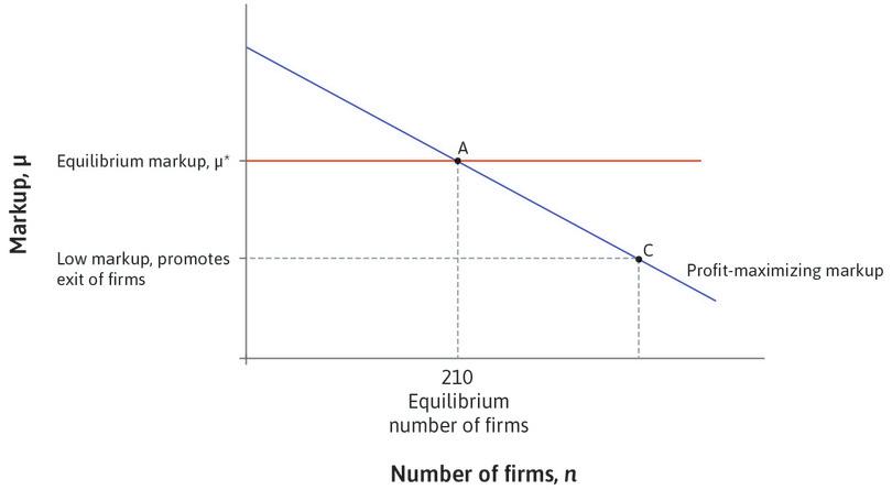
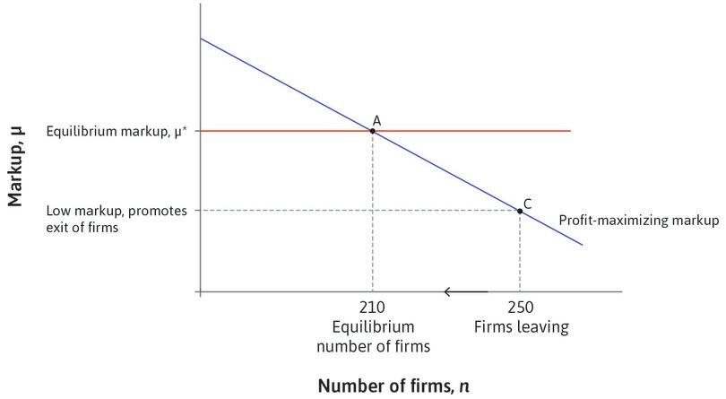
- Firm exit due to a low markup: Owners may withdraw their funds or even close firms if the existing markup is too low, meaning that the expected rate of profit after taxes is not attractive relative to the alternative uses to which the owners could put their assets. These alternative uses could be investing in foreign subsidiaries, outsourcing part of the production process, buying government bonds, or distributing its profits as dividends to the owners. In this case, the number of firms falls.
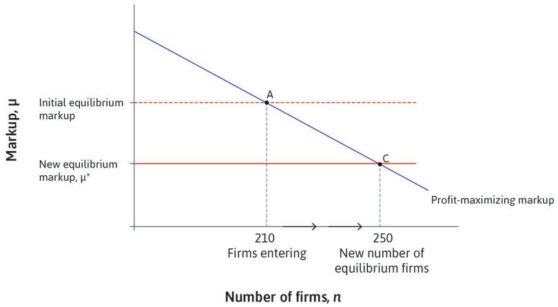
- Firm entry due to a high markup: If the markup is sufficiently high, the resulting high profit rate will attract new firms to enter the economy.
When is firm exit due to too low a markup likely to happen? This will occur when the economy is highly competitive as a result of a great number of competing firms, resulting in a high elasticity of demand for the firm’s products and hence a small markup. When there are ‘too many’ firms to sustain a high enough markup, then firms will exit, which will tend to raise the markup.
Similarly, when there are few firms in the economy, the degree of competition will be limited, the markup will be high, and the resulting profit rate will be sufficient to attract new firms to enter. As a result, the economy will become more competitive and the markup will fall.
This means that the markup has a tendency to self-correct. If it is too low then firms will exit and it will rise, and if it is too high then firms will enter and it will decline.
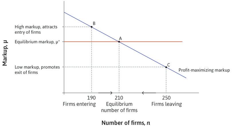
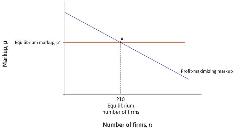
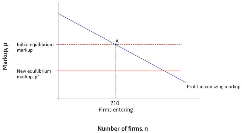
Figure 16.7a illustrates this process by showing how the number of firms and the profit-maximizing markup are related. For each number of firms, the downward-sloping line gives the markup that maximizes the firm’s profits. It slopes downward because:
- The more firms there are, the more competitive the economy is.
- This means a higher elasticity of demand facing the firms when they sell their products (less ‘steep’ demand curves).
- The markup that maximizes the firm’s profits will fall, because, as we saw in Unit 7, the markup, μ, is 1/(elasticity of demand).
The other line in the figure is horizontal and shows the markup that is just sufficient to retain the existing number of firms, which we call μ*. Follow the steps in the analysis in Figure 16.7a to see why the number of firms will be stable at 210.
Now, using Figure 16.7a, think what would occur if as a result of a change of government, the risk of expropriation of private property by the government decreased. This is an improvement in the conditions for operating a business, and could include changes in legislation that reduce the probability that the government will take over firms or implement unpredictable changes in taxation. With better business conditions, a lower markup is required for firms to operate in this economy. Follow the steps in Figure 16.7b to see how this leads to an increase in the number of firms in equilibrium.
From the equilibrium markup to the price-setting curve in the long run
As before, once we know the markup μ* and the average product of labour λ, we know the real wage w that must result: it is the share of the average product of labour (or, equivalently, of output per worker) that is not claimed by the employer through the markup. With constant returns to scale, if capital per worker remains constant, higher employment is consistent with constant output per worker: the long-run price-setting curve is flat. We note as well that in the model, the unemployed and employed workers are identical because of the presence of involuntary unemployment in the labour market equilibrium.
The long-run price-setting curve is given by:
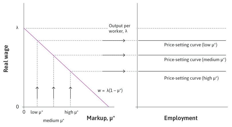
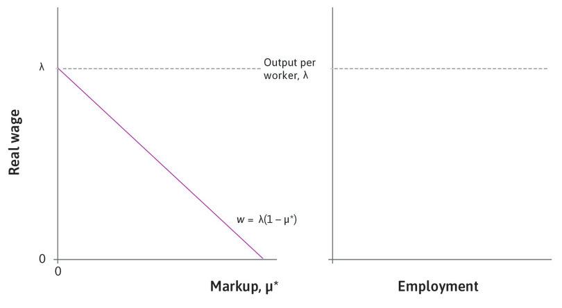
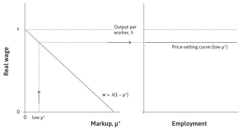
As Figure 16.8 shows, this fact allows us to translate the equilibrium markup into the real wage paid, which fixes the height of the price-setting curve. In the left-hand panel, the equation of the long-run price-setting curve is drawn as a horizontal line, with the equilibrium markup on the horizontal axis and the wage on the vertical axis: with a zero markup, the wage is equal to output per worker; and when the markup is equal to 1 (or equivalently 100%), the wage is equal to zero.
The right-hand panel of Figure 16.8 shows the long-run price-setting curve at different levels of the long-run equilibrium markup. By employment on the horizontal axis in the long-run model, we mean employment with constant capital per worker. We can summarize the factors that will shift the long-run price-setting curve through their effects on either output per worker or the markup.
The long-run price-setting curve is higher:
- the higher the output per worker
- the lower the long-run markup at which firm entry and exit are zero
The long-run price-setting curve
Once we know the equilibrium markup μ* and the productivity of labour λ, we know the real wage w is given by:
w is the output per worker that is not claimed by the employer through the markup.
What lowers the markup at which entry and exit are zero?
- higher competition
- lower risk of expropriation of owners in the home economy
- higher quality environment for doing business: for example, better human capital or infrastructure
- lower expected long-run tax rate
- lower opportunity cost of capital: for example, a lower interest rate on bonds
- lower expected profits on foreign investments
- lower expected long-term cost of imported materials
Exercise 16.4 Measuring the conditions for investment
Go to the World Bank’s Doing Business database.
- In the ‘Topics’ section, collect (download) data on three characteristics of the business environment that will affect the long-run markup, for 20 countries of your choice. Justify your choice of characteristics.
Now go to the World Bank’s DataBank database.
- Download GDP per capita data for the 20 countries of your choice. For each characteristic, create a scatterplot with the characteristic of the business environment (rank) on the horizontal axis, and GDP per capita on the vertical axis. Summarize the relationship between the two variables (if any).
- Explain why a good business environment may raise GDP per capita.
- Why might high GDP per capita improve the business environment?
- From your answers to questions 3 and 4, explain the potential challenges when interpreting the relationship between two variables using a scatterplot.
Question 16.4 Choose the correct answer(s)
Figure 16.8 depicts the graphs of the long-run price-setting curve and the markup at which firm entry and exit are both zero.
Based on this information, which of the following statements is correct?
- An increase in the degree of competition will lower the markup and raise the price-setting curve.
- A lower interest rate means lower opportunity cost of capital. Therefore the profit rate at which firm entry and exit are zero is lower, meaning that the corresponding wage rate (shown by the price-setting curve) is higher.
- Lower worker productivity (λ) causes the real wage-setting curve on the left-hand graph to rotate downwards (pivoted at μ* = 1 on the horizontal axis). This shifts the price-setting curves down for a given μ*.
- This will lower the expected return on investments abroad, lowering equilibrium profits at home and therefore lowering the markup. This leads to a higher price-setting curve.
Question 16.5 Choose the correct answer(s)
Which of the following statements is correct regarding the model of the labour market?
- This is how we define the long run.
- At a given capital stock, labour-saving technological progress raises unemployment, but as the capital stock expands with new firm entry, unemployment falls, and may be lower than initially.
- Firms enter when the markup is high, which means a higher profit rate.
- The markup self-corrects as the firms enter and exit: a high markup leads to more firms entering, resulting in a fall in the markup, while a low markup leads to firms exiting, resulting in an increase in the markup.
16.5 New technology, wages, and unemployment in the long run
We have seen that, contrary to the fears of the Luddites, the constant increase in the amount produced in an hour of work has not resulted in ever-increasing unemployment. It is wages that on average have risen, not unemployment.
In many countries, the combination of technological progress and investment that raises the capital stock roughly doubled the productivity of labour each generation. Our model showed the result: a rise in the real wage that was consistent with profits high enough to motivate firm owners to continue investing, rather than using their wealth in other ways.
The Luddites were right to be concerned about the hardships experienced by those thrown out of work. What they missed is that the additional profits made possible by the introduction of the new technologies provided a kind of self-corrective: additional investments that would sooner or later result in the creation of new jobs.
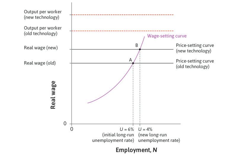
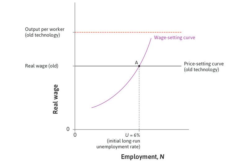
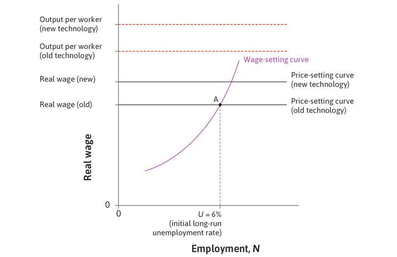
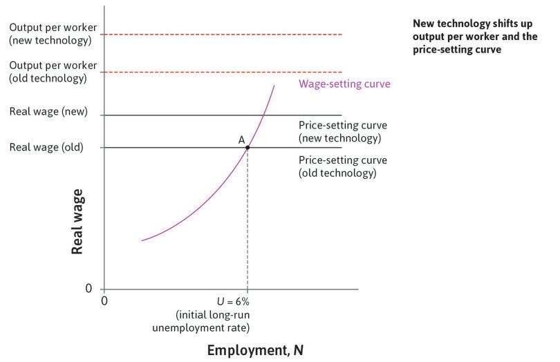
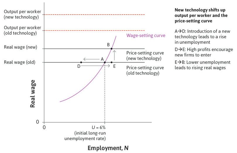
The upward shift in the price-setting curve is illustrated in Figure 16.9a, which shows the status quo (‘old technology’) with the long-run equilibrium at A, and a technological advance that shifts the long-run equilibrium to B. At point B, the real wage is higher and so is the employment rate, in other words, unemployment is lower. The model shows that technological progress need not raise unemployment in the economy as a whole.
Before examining the experiences of unemployment in different countries, we need to understand:
- What determines the rate of increase in the productivity of labour? This accounts for the upward shift in the price-setting curve.
- How does the economy shift from A to B? Both are long-run equilibria in the labour market.
New knowledge and new technology: The innovation diffusion gap
- diffusion gap
- The lag between the first introduction of an innovation and its general use. See also: diffusion.
It often takes years, if not decades, before an improved technology is widely introduced in an economy. This diffusion gap causes differences between the productivity of labour in the most advanced firms and the firms that lag technologically.
In the UK, one study found that the top firms are more than five times as productive as the bottom firms. Similar differences in productivity have been found in firms in India and China. In Indonesia’s electronics industry—a part of the highly competitive global market—data from the late 1990s show that the firms at the 75th percentile were eight times as productive as those in the 25th percentile.
The low-productivity firms manage to stay in business because they pay lower wages to their employees, and in many cases earn a lower rate of profit on the owner’s capital as well. Closing diffusion gaps can greatly increase the speed at which new knowledge and management practices are in widespread use.
This may occur when a union bargains for wages such that equivalent workers are paid the same throughout the economy. One consequence of this is that the least productive firms (which are also those paying low wages) will experience wage increases, making some of these firms unprofitable and putting them out of business. The union might also support government policies that complement its role in hastening the exit of unproductive firms, raising average productivity in the economy and shifting up the price-setting curve. In this case, associations of workers can help bring about creative destruction instead of resisting it.
Associations of owners may also be part of the process of creative destruction by not seeking to prolong the life of unproductive firms, knowing that their demise is part of the process of making the pie larger. But in many cases, employees and owners of the lagging firms do not act in this way. They gain protection through subsidies, tariff protection, and bailouts that guarantee, at least for a time, the survival of the unproductive firm and its jobs.
The rate at which the economy’s price-setting curve shifts upward depends on which of these attitudes towards the process of creative destruction is predominant. Economies differ greatly in this respect.
Adjustment to technological change: The employment and wage adjustment gap
Economies differ too in how they make the journey from the status-quo equilibrium like A to a new equilibrium such as B in Figure 16.9b.
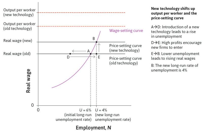
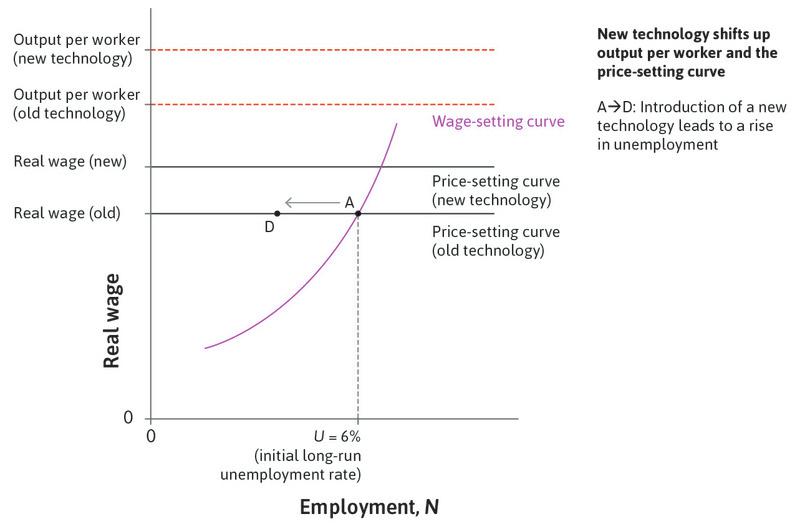
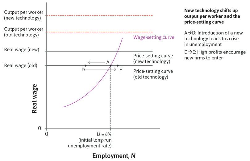
Recall that the price-setting curve in the long-run model is the level of the real wage such that firms will neither enter nor leave the economy. So the move from point A (at 6% unemployment) to point B (at 4% unemployment) occurred because firms entered the economy, a process that takes some time. What happened along the way? Follow the steps in the analysis in Figure 16.9b to see one possible path.
Was this a win-win journey? Only if you compare the start and end points or have a sufficiently long time horizon. The time between the introduction of new technology and the new long-run equilibrium is usually measured in years or even decades, not weeks or months. Younger workers might have more to gain from the eventual higher wages and employment, but older workers might never experience the outcome at B.
Also, note that in Figure 16.9b, we assumed that the real wage did not decline in the short run. But if the economy were to move to point D, firms could lower the real wage so that it lies on the wage-setting curve at the new level of unemployment. This is more likely to happen if the new investment that would take the economy to point E is slow in arriving. In that case, wages may fall under the pressure of greater unemployment before employment adjusts upwards.
We have already seen that in Britain, the adjustment to the technological progress in the eighteenth and nineteenth centuries (the Industrial Revolution) was not rapid. There was a prolonged delay before real wages began to rise continually, starting around 1830.
- adjustment gap
- The lag between some outside change in labour market conditions and the movement of the economy to the neighbourhood of the new equilibrium.
Just as was the case with the diffusion gap, public policies, trade union, and employer association practices can alter the size of this employment and wage adjustment gap. Government policy can help reallocate workers to new firms and sectors by providing job-matching and retraining services, and by providing generous but time-limited unemployment benefits. This helps workers released from failing firms to move quickly to better ones.
The size of these adjustment gaps also depends on institutions and policies that could ease or hamper the creation of jobs in new sectors. If the wage is below the price-setting curve, profits are sufficient to create new investment and form new firms. This is part of the process of adjusting to creative destruction. Some countries have well-designed product-market regulation and competition policy that make it easier to start a new business. In others, incumbent businesses have succeeded in making it difficult for new firms to enter, which slows or even prevents the economy moving to point B.
Looking back at Figure 16.1, you may wonder why the unemployment rate does not shrink continuously in a world with continuous technological progress. The reason is that other forces in the economy lead to the wage-setting curve shifting upwards. Trade unions could be responsible for this shift (as in Unit 9), but there are other explanations:
- Unemployment benefits: Elected members of government may adopt more generous unemployment benefits as the economy adjusts to the new technology. They wish to assist those out of work. This improves the reservation position of workers and shifts the wage-setting curve up.
- Rural wages: Technological improvements in the countryside and migration from rural areas to cities associated with the implementation of new technology in manufacturing may raise rural incomes and therefore increase the workers’ reservation option, which lowers the cost of losing a manufacturing job. As a result, urban employers must pay more to induce employees to work. This situation could occur in developing countries with large rural sectors.
We further explore these forces in Unit 17, when we investigate the golden age of capitalism following the Second World War.
Lessons from creative destruction and consumption smoothing
By this time, you may have noticed two recurring themes in this course:
- Creative destruction: Improvements in living standards often occur by a process of technological progress in which jobs, skills, entire sectors, and communities become obsolete and are abandoned. We study this process in Units 1, 2, 16, and 21.
- Consumption smoothing: Households faced with shocks to their income seek to even out the ups and downs of their standard of living through borrowing, unemployment benefits, mutual assistance among family and friends, and other forms of co-insurance. We studied this process in Units 10, 13, and 14.
The two themes above are related. People suffering from job destruction will suffer less if they can smooth their consumption. Economies differ greatly in the extent to which their policies, culture, and institutions allow consumption smoothing. In those that do this well, resistance to the creative-destructive forces of technological progress is likely to be low. In those that do not, owners and employees alike will try to find ways to resist (or halt) the process of creative destruction, preferring to defend their firm’s assets and existing jobs.
The attitude of unions to the process of job destruction and creation is an example. In countries with adequate consumption-smoothing opportunities, trade unions tend not to insist on a worker’s right to keep a particular job. Instead they demand adequate new job opportunities, and support in searching and training for new work.
- employment protection legislation
- Laws making job dismissal more costly (or impossible) for employers.
In other countries, unions and government policy seek to protect the status quo matching of workers to jobs, for example by making it more difficult to terminate a labour contract, even when the worker has performed inadequately. This employment protection legislation may be harmful to labour market performance by enlarging the diffusion and adjustment gaps, and slowing the rate of technical progress, while at the same time pushing the wage-setting curve up.9
These differing responses to the opportunities and challenges presented by creative destruction will help us understand why some economies performed better than others in recent history.
Question 16.6 Choose the correct answer(s)
Watch our ‘Economist in action’ video featuring John van Reenen about the determinants of the productivity of firms. Based on the video, which of the following statements is correct?
- Different management practices are part of the explanation, but do not entirely explain the huge variation. Technology and the rate of innovation diffusion is another important determinant.
- While a country’s openness to FDI is an important factor for improving productivity, the video did not suggest that it is more important than creative destruction.
- Driving up average productivity through new entry and innovation (the ‘creative’ part) takes time and the effects can usually only be seen in the long run. The closure of low productivity plants will raise average productivity in the short run, a phenomenon sometimes referred to as the ‘batting average’ effect.
- Openness to imports affects the flow of new ideas into the economy, which can promote technological advances and innovation.
Question 16.7 Choose the correct answer(s)
Figure 16.9b depicts the long-run adjustment process in the labour market after technological progress.
Based on this information, which of the following statements is correct?
- In the short-run, initially there is a displacement of some workers from their jobs, which increases unemployment, as shown by the movement from point A to point D.
- Firms increase investment due to the large gap between the old real wage (solid line) and the new output per worker (dashed line), which implies higher profits.
- E is below the wage-setting curve so workers need a higher wage to be induced to work.
- The adjustment to the new equilibrium requires entry of new firms, which can take a substantial amount of time.
16.6 Technological change and income inequality
- short run (model)
- The term does not refer to a period of time, but instead to what is exogenous: prices, wages, the capital stock, technology, institutions. See also: price, wages, capital, technology, institutions, medium run (model), long run (model).
- long run (model)
- The term does not refer to a period of time, but instead to what is exogenous. A long-run cost curve, for example, refers to costs when the firm can fully adjust all of the inputs including its capital goods; but technology and the economy’s institutions are exogenous. See also: technology, institutions, short run (model), medium run (model).
What happens to the distribution of income in an economy when a new technology is introduced that raises the productivity of labour? Think about the case we just studied in Figures 16.9a and 16.9b, where we highlight the contrast between the short-run immediate impact, and the long-run outcome that results once the higher profits, made possible by the innovation, have motivated additional investments by firm owners.
In the short run, the economy moves from point A to point D in Figure 16.9b. The new technology raises output per worker and reduces the number of people employed. For those employed at D, we assume that in the short run the real wage is unaffected.
What is the effect on inequality in the short run, at point D? Inequality increases for two reasons: first, because of the rise in the number of unemployed workers with low or no income, and second because in the short run only the employers reap the benefit of the new technology. The employers’ share of output goes up. This is summarized in the first row of Figure 16.10. Of course, had wages at D fallen to meet the wage-setting curve at the new unemployment rate, this would have exacerbated the rise in inequality.
But this is not where the process ends. Point D in Figure 16.9b is not a Nash equilibrium because at the new level of productivity and the old real wage, firms are making sufficient profits to either attract new firms to enter or to incentivize existing firms to expand their output. Looking back to Figure 16.9b, the economy expands and more people are employed. This also pushes wages up along the wage-setting curve. This process will continue until the wage is sufficiently high that firms stop expanding or entering the economy, that is until the economy reaches point B, the new Nash equilibrium.
| In Figure 16.9b | Employment | Unemployment | Wage share | Inequality | |
|---|---|---|---|---|---|
| Short run (number of firms and their capital stock do not change) | A to D | Down | Up | Down | Up |
| Long run (outcome adjusts fully to the new Nash equilibrium of the model, no change in wage-setting curve) | A to B | Up | Down | No change | Slightly down |
Effects of technological improvements on the labour market model: Short and long run.
Figure 16.10 Effects of technological improvements on the labour market model: Short and long run.
Comparing the new Nash equilibrium at point B with the initial one at point A, both workers and employers benefit from the new technology. The wage share is back at its initial level and inequality is lower at B because the unemployment rate is lower. Note that although the wage share at B is no higher than at A, real wages are higher.
The long-run effect of the change in technology was to slightly reduce inequality because:
- the share of output going to employees was restored to its pre-existing level in the long run due to an increase in real wages
- the higher real wage allowed employers to maintain motivation for workers to work hard at a lower level of unemployment
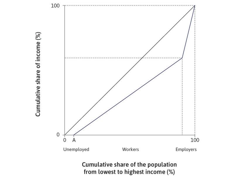
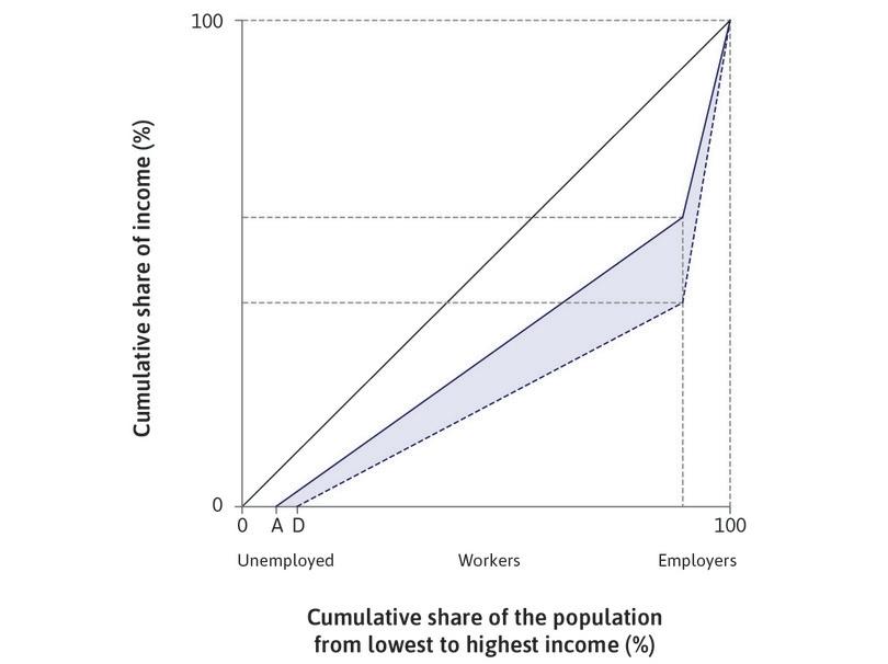
To see the effect on inequality, we will represent the initial situation by a Lorenz curve (introduced in Unit 5 and used also in Units 9 and 10), and then see how its shape changes. In Figure 16.11, the unemployed, workers, and employers are shown on the horizontal axis.
The solid line in Figure 16.11 is the Lorenz curve corresponding to the situation at point A in Figure 16.9b. When unemployment increases to D (on the horizontal axis), the Lorenz curve shifts out to the dashed one. The kink is lower, reflecting the lower wage share at point D. In the long run, unemployment falls to B and the wage share returns to its initial level. The Lorenz curve shifts inwards.
Follow the steps in the analysis in Figure 16.11 to see how the Lorenz curve changes on the way to the new equilibrium.
Exercise 16.5 Technological progress and inequality
The Einstein in Unit 9 showed that the Gini coefficient g can be calculated from the three groups of people in the economy-wide labour market as follows:
Here, u represents the fraction unemployed, n the fraction of the labour force in employment, the quantity 1 − n − u the fraction of the labour force that are employers, w the real wage, and λ the output per worker. The expression w/λ is the fraction of total output that workers’ wages can purchase, called the wage share. This is clear because wn is total wages paid, and λn is total output produced.
In the initial Lorenz curve (prior to the technical change), suppose there were 6 unemployed, 84 employed workers and 10 employers, with wages sufficient to purchase 60% of output.
- Confirm that the Gini coefficient in this case would be 0.336.
- Now suppose that technological progress leads to 4 workers losing their jobs while output stays constant, and the wage level of the remaining workers also stays constant, so profits increase by the amount that the total wage bill has dropped. What is the new wage share? What is the new Gini coefficient?
- In the long run, assume there are 4 unemployed, 86 employed, and 10 employers, and the wage share returns to 60%. What is the Gini coefficient now? In your own words, explain why inequality increased in the short run and fell in the long run.
Question 16.8 Choose the correct answer(s)
Does the introduction of a new labour-saving technology results in …?
- The labour-saving technology leads to higher unemployment while the wage and total output are constant. This means that the profit share of output is higher, and the wage share is lower. The Gini coefficient is higher.
- The increase in unemployment lowers total wages and hence the wage share in the economy.
- Higher unemployment with constant wages and total output lowers the wage share of output but increases the Gini coefficient.
- In the long run, improvements in technology result in job creation too, leading to lower unemployment. The wage share remains constant because the markup is constant, and the Gini coefficient is lower.
16.7 How long does it take for labour markets to adjust to shocks?
How long is the long run? In 1923, John Maynard Keynes wrote:
The long run is a misleading guide to current affairs. In the long run we are all dead. Economists set themselves too easy, too useless a task if in tempestuous seasons they can only tell us that when the storm is past the ocean is flat again. (A Tract on Monetary Reform)10
What you think about Keynes’ quote, especially the italicized part, may depend on your age (he was 40 at time and would live another 23 years). The sea is flat in equilibrium, in Keynes’ metaphor, but if you are interested in safe navigation what may be more important is what happens in the passage from one equilibrium to another, in other words, getting through the storm. Keynes advocated what we have earlier termed a dynamic view of the economy, that is, one that focuses on changes.
In Section 16.5 we studied how, if the labour market is knocked out of equilibrium by a labour-saving innovation that puts employees out of work, there may be a new long-run equilibrium in which the displaced workers are re-employed at higher wages. Keynes’ point is that good economic policies have to be based on an understanding of how the economy gets from one equilibrium to the other and how long it takes.
But many economists since have taken what Keynes called the ‘easy’ approach and just focused on one or more equilibria. When something changes (like a new technology), economists compare the equilibrium before and after the change. This is termed the comparative static approach (static means unchanging, so the idea is to compare two things that are different–the before and after–but are themselves static.)
Hal Varian (1947– ), an important American economic theorist, points out the difficulties in knowing what happens out of equilibrium and so tells the readers of his popular microeconomics text: ‘we will generally ignore the question of how the equilibrium is reached, and focus only on the issue of how firms behave in the equilibrium.’
Varian is right: it is important to know what happens in equilibrium and how the level of employment, wages, and profits that occur in equilibrium will differ depending on conditions and policies adopted. It is also not true that in the long run ‘we’ are all dead, unless the only people you count as ‘we’ are those alive now, not future generations who will live after you and experience the long run effects of the policies adopted now. And we know from Unit 4 that people do care about the wellbeing of others, so the long run matters even if it is very long.
If when things change, the economy moves quickly from one equilibrium to another, the comparative static approach advocated by Varian makes sense. If the process of equilibration takes a long time or if we cannot even be sure that the economy will move to another equilibrium (see ‘Do bubbles exist?’ in Unit 11), then Keynes’ emphasis on the dynamics of the adjustment process seems appropriate.
In Unit 11 we explained that when a market is not in equilibrium, there are opportunities for economic actors to benefit by changing the price or quantity they are selling or buying. These so-called rent-seeking activities are part of the process by which a new equilibrium is established. In a fish market, for example, rent seeking just means offering or charging a different price, and the process of getting to a new equilibrium is relatively quick.
But in the labour market, if competition from other firms has reduced the demand for the good you are producing and put you out of work, the process is going to be slower. The reason is that the rent seeking that may bring about a new equilibrium may involve you retraining to develop a new set of skills, or you may have to uproot your family and seek work in a new location.
The debate on how quickly the US labour markets would adjust to the ‘shock’ of competition from imports of manufactured goods from China is a case in point. Around the turn of the current century after more than a decade of rapidly rising imports from China, there was a consensus among US economists that imports were not having any major negative effect on wages or employment, in part because workers producing goods competing with imports could easily relocate to other regions. In another of our earlier ‘Economist in action’ videos on global production and outsourcing, Richard Freeman asked if wages in the US were ‘being set in Beijing’ and answered with a resounding ‘no’.
Yet evidence was accumulating even then that the adjustment of the US economy to the China shock was not going to be a simple textbook comparative static jump from one equilibrium to another. Most economists did not then anticipate the extent to which China would quickly come to dominate global production of manufactured goods: having produced one-twentieth of the world’s manufactured goods in 1990, a quarter of a century later it produced a quarter of the global total.
But it was not just the unexpected size of the China shock that overturned the optimism of many economists; the labour market’s adjustment did not work as quickly as they had assumed.
The impact on US labour markets was geographically concentrated: parts of the state of Tennessee specializing in furniture production and facing competition from China were hard hit, while nearby Alabama specializing in heavy industry was barely affected since China did not export heavy industrial goods. The geographical concentration of the effects of the China shock has allowed economists to study how labour markets adjusted.11
They found that in US labour markets, the long run is a very long time. ‘China exposed’ regions suffered major losses in manufacturing employment; many of the jobless found it impossible to find work locally and gave up, they left the labour force. Very few left the region. Localities hit by import competition in the 1990s continued to be depressed into the second decade of this century. Between 1999 and 2011, the China shock led to a loss of 2.4 million jobs.
The conclusion of a major study of the China shock sounded more like Keynes than Varian. If one had to project the impact for the US labour market with nothing to go on other than a standard undergraduate economics textbook, one would predict large movements of workers between US tradable industries (meaning, exporting or competing with imports), for example, from apparel and furniture to pharmaceuticals and jet aircraft. You would also expect limited reallocation of jobs from tradables to non-tradables, and no net impacts on US aggregate employment. The reality of adjustment to the China trade shock has been very different.
Adjustment to the introduction of labour-saving machinery, which we have studied in this unit, is likely to be similarly slow. In Unit 18 we return to China in the world economy, and show that the response to the China shock in Germany was quite different.
16.8 Institutions and policies: Why do some countries do better than others?
What do we mean by ‘good’ performance or a ‘good’ outcome? The answer matters because citizens who vote for parties with alternative economic programs, and policymakers who attempt to improve those programs, will need some concept of what is desirable—either for the individual, the policymaker, or the nation.
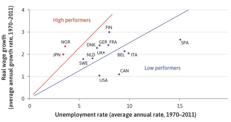
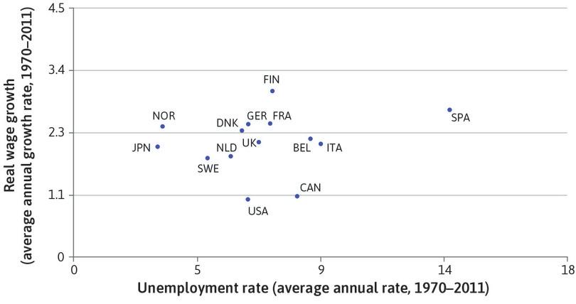
As we saw in Unit 3, people value their free time as well as their access to goods. We should include their reward per hour of work in our evaluation of outcomes. In any given year, a ‘good’ performance is one in which unemployment is low and real wages per hour are high. Putting this into a dynamic setting, and evaluating an economy over many years, we judge performance as ‘good’ if a country combines rapid growth of real wages per worker hour with low unemployment.
There are of course other dimensions of long-run economic performance that most people care about. We may care whether or not the distribution of economic rewards is fair, whether or not the economy’s relationship with the natural environment is sustainable, or about the extent to which households are subjected to economic insecurity through business cycle fluctuations. But here we focus solely on the growth in real wages per hour and the unemployment rate.
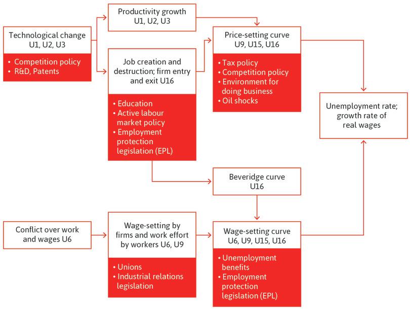
We use the labour market model and the Beveridge curve to see that achieving good performance requires an economy to have two capacities:
- To raise the price-setting curve and restrain the upward shift of the wage-setting curve: So that both hourly wage growth and the long-run employment rate are high.
- To adjust rapidly and fully: So that the entire economy can take advantage of opportunities from technological change.
Technological change means jobs disappearing in firms in which new technology substitutes for workers. Jobs also disappear as new firms enter and those unable to adapt to the new conditions shut down. The Beveridge curve highlights the importance of matching workers and vacancies in the labour market. In Figure 16.9b, we saw that the impact of new technology is initially to displace workers: the Beveridge curve summarizes the economy’s ability to rapidly redeploy displaced workers, shortening the period the economy spends in the short-run situation (point D, Figure 16.9b).
Figure 16.12 shows long-run performance (over a 40-year period) for a group of advanced economies. It uses the criteria of real wage growth and unemployment rates. We study a long period because we do not want our evaluation of long-term performance to be affected by the particular phase of the business cycle in which a country finds itself (it will look much better at the peak than at the trough). We use wages in manufacturing because they are measured in ways that are more accurately comparable across nations—although this is not ideal, because the share of employment in manufacturing shrinks over time and varies across countries.
Good performance places a country in the top-left corner of Figure 16.12, with high wage growth and low unemployment; bad performance places a country in the bottom-right corner. Since we value both high wage growth and low unemployment, we may be prepared to tolerate low wage growth if it is associated with a lower level of unemployment. This means that we can represent a citizen’s indifference curve as a ray from the origin. Steeper rays are better, and a country’s performance is measured by the steepness of a ray from the origin to that country’s observation. If you look at Figure 16.12, and take Belgium (BEL) as an example: a Belgian citizen would prefer to be on a steeper ray, like that of Germany (GER), with lower unemployment and higher wage growth.
Long-run unemployment and real wage growth across the OECD (1970–2011).
Figure 16.12 Long-run unemployment and real wage growth across the OECD (1970–2011).
OECD. 2015. OECD Statistics; BLS data for Spanish real wages available only from 1979. Spanish real wage growth for 1970–1979 has therefore been estimated using Tables 16.25 and 16.5 from Barciela López, Carlos, Albert Carreras, and Xavier Tafunell. 2005. Estadísticas históricas de España: Siglos XIX-XX. Bilbao: Fundación BBVA.
The two rays in Figure 16.12 divide the countries into three groups. The high performers over the 40-year period from 1970 to 2011 are Norway and Japan. The low performers are Belgium, Italy, US, Canada, and Spain. The poor performance of the US is in part due to the fact that it started with higher wages in 1970, because it was the world’s technology leader during this period (as we saw in Figure 16.3). This meant that other nations could learn from it, rapidly raising their productivity. Similar arguments apply to Canada. For this reason we do not take these two countries as representative of the low performers, although real wages have grown much more slowly than productivity in the US, so most US citizens did not benefit very much from economic growth in this period.
Notice that successful countries used different combinations of policies and institutions. Some of the best performers (on steeper rays from the origin) like Norway, Finland, Sweden, and Germany have powerful unions, while the Nordic countries (including Denmark) have some of the most generous unemployment benefits in the world.
Figure 16.13 reproduces the unemployment data from Figure 16.1, but with two of the high performers and two of the low performers from Figure 16.12 highlighted. The differences between Japan and Norway on one hand, and Italy and Spain on the other, centre on unemployment rather than real wage growth. In Figure 16.13 you can see how unemployment behaved differently following the oil shocks of the 1980s, and after the financial crisis.
Unemployment rates of two high and two low labour market performers (1960–2014).
Figure 16.13 Unemployment rates of two high and two low labour market performers (1960–2014).
Data from 1960–2004: David R. Howell, Dean Baker, Andrew Glyn, and John Schmitt. 2007. ‘Are Protective Labor Market Institutions at the Root of Unemployment? A Critical Review of the Evidence’. Capitalism and Society 2 (1) (January). Data from 2005 to 2012: OECD harmonized unemployment rates, OECD. 2015. OECD Statistics.
We shall see that the model in this unit provides a useful framework for understanding the high and low performers of the labour market. We will now show how to use the model to explain the way that institutions and policies affect real wage growth and unemployment in the long run.
Exercise 16.6 You are the policymaker
Refer to Figure 16.12 to answer the following questions:
- Using the same axes, draw the indifference curves of a citizen or policymaker who cares only about wage growth.
- According to the data in the figure, which countries would be the high performers and which would be the low performers?
- Using the same axes, draw your indifference curves if you only cared about the unemployment rate. Which countries would be the high and low performers in this case?
- Using the same axes, draw an indifference curve based on your own personal preferences over wage growth and unemployment, and justify your choice.
- Now considering your preferences over other economic factors, which country in the figure would you choose to live in, and why? Explain which economic factors you included in your decision.
Question 16.9 Choose the correct answer(s)
The following graph plots the real wage growth of different countries against their unemployment rate, averaged over the period 1970–2011.
Based on this information, which of the following statements is correct?
- Japan is the country that has managed to keep its unemployment the lowest across the period.
- All the European countries in the figure have had higher wage growth.
- Spain has managed high wage growth, but with high unemployment.
- Although Finland managed higher wage growth, it also had high unemployment. If the citizens’ indifference curves are given by straight lines from the origin, then in fact Norway’s performance would be on a higher indifference curve.
16.9 Technological change, labour markets, and trade unions
Policies and institutions make a difference. The models shed light on the experience of some of the best and worst performers. We take three countries as examples: Norway and Japan as good performers, and Spain as a poor performer.
In Norway and Spain, unions are important, but not in Japan. In Norway, more than half of all wage and salary workers are trade union members, and union wage deals affect most workers in the economy. In Spain, although union wage deals are important for the entire economy, less than one-fifth of Spanish workers are in unions.
Union wage bargaining coverage and unemployment across the OECD (2000–2014).
Figure 16.14 Union wage bargaining coverage and unemployment across the OECD (2000–2014).
OECD. 2015. OECD Statistics. Labour force statistics. Visser, Jelle. 2016. ‘ICTWSS: Database on Institutional Characteristics of Trade Unions, Wage Setting, State Intervention and Social Pacts in 51 countries between 1960 and 2014’ Amsterdam Institute for Advanced Labour Studies (AIAS).
Figure 16.14 provides information on the importance of union wage deals and unemployment. On the horizontal axis, we plot the percentage of employees whose wages are determined by union wage deals. As you can see, in some European countries, union wage deals cover almost all employees. And in the set of countries with coverage of more than 80%, unemployment rates range from less than 4% (Netherlands) to almost 14% (Spain). Figure 16.14 suggests that there is no tendency for unemployment to be higher in countries in which unions are more influential in wage-setting. Low unemployment is found in countries extending across the whole range of union strength. Compare South Korea and the Netherlands, Japan and Austria, or the US and Sweden.
Just as the employer does not offer the lowest wage possible, most unions do not seek the highest wage they could win in bargaining. Employers offer wages above the minimum because they cannot control how hard the worker works. Unions do not bargain for the maximum wage possible (the wage that would leave none of the pie for the owners) because unions cannot control the firm’s decisions about hiring, firing, and investment, and higher wages may reduce employment by reducing the firm’s profits.
- medium run (model)
- The term does not refer to a period of time, but instead to what is exogenous. In this case capital stock, technology, and institutions are exogenous. Output, employment, prices, and wages are endogenous. See also: capital, technology, institutions, short run (model), long run (model).
A union organized across many firms and sectors will not exploit all the bargaining power it possesses. It knows that large wage gains will lead to:
- In the medium run: Restrictive aggregate demand policies, as the government and central bank seek to keep inflation close to target (as we saw in Unit 15).
- In the long run: The exit of firms and a smaller stock of capital goods, which will slow the rate of productivity growth.
- inclusive trade union
- A union, representing many firms and sectors, which takes into account the consequences of wage increases for job creation in the entire economy in the long run.
Unions that act this way are called inclusive trade unions. Non-inclusive unions may bargain for high wages in their own corner of the economy without regard for the effects on other firms or workers, both employed and unemployed. Employers’ associations that take account of the interests of all businesses, including those that might enter an industry and compete with its incumbent firms, are called inclusive business or employers’ associations. When unions and businesses act in an inclusive manner there is also more likely to be a positive union voice effect. As discussed in Unit 9, this lowers the disutility of work, helping to push down the wage-setting curve.
The Nordic case: Inclusive unions and employers’ associations
This inclusive behaviour is exactly what the trade unions and employers’ associations of Norway (as well as in the other Nordic countries) did over this period: their centralized wage bargaining insisted on a common wage for a given kind of labour, depriving low-productivity firms of access to inexpensive labour and driving many of them out of business. As workers were quickly redeployed to employment in more productive firms, the main impact was to raise average labour productivity, pushing up the price-setting curve and allowing higher wages.
Inclusive trade unions also support generous income floors and high-quality publicly provided healthcare, occupational retraining, and educational services—all of which reduce the risk to which most individuals are exposed. This has the effect of making the creative destruction of technological change less destructive for people’s personal lives and allows them to be generally more open to change and to risk-taking. Both of these attributes are essential for a technologically dynamic society.12
These so-called ‘active labour market policies’ improve the matching process between workers looking for work and job vacancies available for workers. A result is that workers whose jobs are eliminated (for example, by the failure of low-productivity firms under the pressure of centrally bargained uniform wages) can find an alternative job more quickly. The result is a Beveridge curve closer to the origin, superior to both the German and US Beveridge curves (shown in Figure 16.6). It is far inside that of Spain, as we see in Figure 16.15.
Beveridge curves for Spain and Norway (2001 Q1 – 2013 Q4).
Figure 16.15 Beveridge curves for Spain and Norway (2001 Q1 – 2013 Q4).
OECD Employment Outlook: OECD. 2015. OECD Statistics.
An inclusive union knows that the economy has to respect the two major incentive problems of a capitalist economy: providing incentives for workers to work and for employers to invest. In some cases—for example, in Sweden with its highly centralized trade union federation—trade union leaders knew and persuaded their members that in the long run, pushing down the wage-setting curve will increase employment and will not reduce wages.
As a result, the inclusive unions of the Nordic countries (Norway, Sweden, Finland, and Denmark) set their wage demands in accordance with the productivity of labour. When it rose they demanded a fair share. They had bargaining power from low unemployment, high membership, and their ability to implement wage agreements across the economy, but they did not use this power to push the wage-setting curve up unless it was warranted by productivity growth. These unions also supported legislation and policies that make working less onerous, shifting downward the wage-setting curve, and further expanding long-run employment.
The Japanese case: Inclusive employers’ associations
In contrast to the Nordic countries, Japanese unions are weak, but workers are well organized in the large companies. Employers’ associations are strong and work to coordinate wage-setting among the large firms. These associations therefore operate in a similar way to the unions in Norway: the impact of wage decisions on the economy as a whole is taken into account when wages are set. Specifically, the corporations deliberately do not compete in hiring workers, so as to avoid raising wages.
The Spanish case: Non-inclusive unions
Unions protect jobs in Spain, supported by government policy. Wage-setters in Spain are strong enough to wield power, but are not inclusive. A combination of non-inclusive unions and supportive government legislation that protects jobs may help to account for the poor performance of the Spanish labour market.
Based on the model, we would predict high unemployment in Spain, and low unemployment in Norway and Japan. And that is what we see in the data.
Unemployment benefits and unemployment
- gross unemployment benefit replacement rate
- The proportion of a worker’s previous gross (pre-tax) wage that is received (gross of taxation) when unemployed.
The employment-enhancing effects of inclusive trade union and government co-insurance policies may help to explain an apparent anomaly: countries with generous unemployment benefits do not have higher rates of unemployment (see Figure 16.16).
Unemployment benefit generosity and unemployment rates across the OECD (2001–2011).
Figure 16.16 Unemployment benefit generosity and unemployment rates across the OECD (2001–2011).
OECD. 2015. OECD Statistics.
This is anomalous, because in our model an increase in the unemployment benefit would, ceteris paribus, reduce the workers’ cost of job loss, and shift the wage-setting curve up.
The contrast between unemployment rates and benefits in Norway and Italy illustrates the point. An unemployed person gets a benefit of almost 50% of previous gross earnings in Norway, and unemployment is low; in contrast, benefits in Italy offer a 10% gross replacement rate, and unemployment is much higher than in Norway. The implication is that countries that are able to implement generous but well-designed unemployment insurance schemes, coordinated with job placement services and other active labour market policies, can achieve low rates of unemployment. Providing people with opportunities to smooth consumption may make them readier to embrace new technology, which will shift the price-setting curve upward.
Exercise 16.7 Unemployment rates and labour market institutions
Some people have argued that high unemployment in some European countries relative to the US during the 1990s and 2000s was due to the existence of rigid labour market institutions (for example, powerful unions, generous unemployment benefits, and strong employment protection legislation).13
- Using Figure 16.1, check if the unemployment rate has always been higher in most European countries compared to the US.
- From what you have learned from this section, and by looking at Figures 16.1, 16.14, and 16.16, evaluate the claim that high unemployment in Europe was due to the existence of rigid labour market institutions.
Question 16.10 Choose the correct answer(s)
The following is a plot of unemployment rate and trade union density for the period 2000–2012. Trade union density is defined as the fraction of employees who are union members.
Based on this information, which of the following statements is correct?
- Korea has very low trade union density but manages to have a low unemployment rate.
- Czech Republic has a similar trade union density as Slovakia but has a low unemployment rate.
- For Norway, Denmark, Sweden, and Finland, the correlation between the unemployment rate and trade union density is positive, that is, the unemployment rate is higher despite having higher trade union density.
- Lower unemployment in Norway, despite the same high rate of union density, suggests that unions are more inclusive there than in Belgium.
16.10 Changes in institutions and policies
We have seen that differences in institutions and policies make a big difference for employment and wage growth, and that citizens of Spain might wish to have institutions like those of Japan or a Nordic country. But changing institutions is difficult because it inevitably creates winners and losers.
Countries that changed their policies changed their fortunes. Both the UK and the Netherlands suffered sharply increased unemployment rates in the 1970s and early 1980s due to the first and second oil shocks (which shifted the price-setting curve down) and the increased bargaining power of labour (which shifted the wage-setting curve up). These effects are illustrated in Figure 16.17. But a change in policy eventually turned the bad news around. In the UK, the unemployment rate fell from 11.6% in 1985 to 5.1% in 2002, and in the Netherlands it fell from 9.2% to 2.8% over the same period.
Different ways of pushing down the wage-setting curve: The Netherlands and the UK.
Figure 16.17 Different ways of pushing down the wage-setting curve: The Netherlands and the UK.
David R. Howell, Dean Baker, Andrew Glyn, and John Schmitt. 2007. ‘Are Protective Labor Market Institutions at the Root of Unemployment? A Critical Review of the Evidence’. Capitalism and Society 2 (1) (January). Data from 2005 to 2012: OECD harmonized unemployment rates, OECD. 2015. OECD Statistics.
Both countries turned around their economies and shifted the wage-setting curves down, but they used different institutions and policies:
- In the Dutch case: Institutions became more inclusive, moving in a Nordic direction by common agreement.
- In the British case: Policy reduced the power of the non-inclusive unions and increased competition in labour markets.14
In the Netherlands, a key component was an agreement in 1982 between employers and unions called the Wassenaar Accord. Unions offered wage restraint (a downward shift in the wage-setting curve) and in exchange, the employers agreed to a reduction in working hours. The union agreed that the reduction in working hours would not increase labour costs (and hence would not shift the price-setting curve down).
In the Dutch case, unions and employers’ associations were capable of coordinating wage-setting to achieve a better macroeconomic outcome. They were powerful enough that they could ensure their members stuck to the agreement. The unions were exercising bargaining restraint in the interests of improved performance of the labour market, and hence in the economy as a whole.
In the UK, the wage-setting curve also shifted down but in this case, it was because of a fall in union power brought about by changing industrial relations legislation, which weakened the ability of the non-inclusive unions to organize strike action.
Exercise 16.8 The labour market model
Explain how to use the labour market model (wage-setting curve and price-setting curve) to show the changes in labour market performance of the UK and the Netherlands from the early 1970s to the early 2000s, as discussed in this section. The article by Nickell and van Ours (2000) referenced above is a good research resource for this question.
16.11 Slower productivity growth in services, and the changing nature of work
The rise and fall of manufacturing employment
As discussed in Unit 1, before the Industrial Revolution most of the output of the economy was made by family members. They were not employees but instead were independent producers of the goods and services both for their own use (called home production) and for sale to others. The Industrial Revolution and the emergence of the capitalist economic system shifted labour from the family and the farm to firms: independent producers became employees.
- industry
- Goods-producing business activity: agriculture, mining, manufacturing, and construction. Manufacturing is the most important component.
Due to technological progress in machine-based production, manufactured goods became cheaper. As a result, textiles and clothing once produced in the home were now purchased and paid for with the wages gained through industrial and other employment. The result was a sustained increase in employment in the industrial sector of the economy. Manufacturing makes up most of the employment in industry, and the terms manufacturing and industry are often used interchangeably.
Labour-saving innovation also made farming more productive. And as people became richer they spent less of their budget on food. Therefore the fraction of the labour force engaged in farming fell.
For many, the shift out of farming and the rise of manufacturing employment meant an improvement in economic opportunities, especially when the trade unions and worker-based political parties forced employers to improve industrial working conditions.
This did not last forever though. Figure 16.18 shows that for most of the world’s large economies, the era of expanding manufacturing employment ended sometime in the third quarter of the twentieth century. Just as manufacturing had initially displaced agriculture as the main kind of employment, the production of services rather than goods has replaced manufacturing. Follow the steps in the analysis in Figure 16.18 to see how major industrial economies passed through stages of rising and falling manufacturing employment at different times.
The economics of slower productivity growth in services
The amount of labour devoted to agriculture has declined in all of the countries shown in Figure 16.18. Fewer than one in 20 workers in rich countries work in agriculture. The recent big shift in work has been from the production of goods (manufacturing and agriculture) to the production of services. We know that output per hour of labour (productivity) is growing more slowly in the production of services than in manufacturing. This has two effects:
- An employment shift: To produce the same mix of goods and services it now takes relatively less labour devoted to goods and more to services.
- A consumption shift: The costs of producing goods have fallen relative to the costs of producing services, and so the prices of goods have fallen relative to the prices of services. This leads people to buy more goods and fewer services than they otherwise would have done.
The first of these effects has been stronger than the second.
To see how this process works, let’s simplify by using a model in which only the first effect occurs. So we assume that people consume a given ratio of goods (shirts, for example) and services (haircuts). The examples illustrate the reason for slower productivity growth in services: it takes about as long today to cut someone’s hair as it did 100 or even 200 years ago, but to produce a shirt it takes much less time than it did 200 years ago (probably less than a fifth).
Figure 16.19 shows the model. The total amount of labour employed in the economy is assumed to be 1 (it could be 1 million hours, for example). If all of this labour is devoted to the production of goods, 1 unit of goods is produced. And the same is true of services: if all the labour produces services, then 1 unit of services is produced.
The solid red line is the feasible frontier, showing the amounts of goods and services that are possible given the existing technologies and the amount of labour employed. We assume that the same number of units of goods and services are consumed, so in the figure the quantity of services and the quantity of goods consumed both equal half a unit in the first period. In the second period, productivity rises in manufacturing while staying constant in services, meaning that the cost and hence the price of goods declines relative to services. Follow the steps in the analysis to see the effect on employment.
Labour has shifted from goods production to services production. This model is designed to illustrate why the shift took place. Two things left out of the model have, in reality, reduced the shift, and a third one has increased it:
- Productivity increases in some services reduces the shift: We assumed that there was no productivity increase in services. But think of the kinds of services we have discussed in this unit, such as the sharing of music or other forms of digital information, where the productivity advances have been large. If productivity in services increased, then in our model it would at least partially offset the shift in labour. We will see just below, however, that much of the service sector of the economy is made up of such things as personal care, which is more like haircuts than the reproduction of music.
- Substitution of goods for services reduces the shift: We increase the proportion of goods we consume if their relative price falls. By assuming that the ratio of goods (shirts) to services (haircuts) did not change, we ignored this process. It would partially offset the decline in goods employment.
- An increase in relative demand for services increases the shift: We also ignored the possibility that as incomes rise, people choose to spend more of their budget on services. Remember that services include tourism and other forms of recreation, and also include health, education, and care, which may not be paid directly out of the household’s disposable income. This would reinforce the shift of labour into services. We have seen this before: it is equivalent to the earlier shift of labour out of agriculture that occurred when the share of food in household budgets shrank.
However, in the countries showing a decline in goods employment relative to services, the net effect of the things we have excluded from the model did not completely offset the deindustrialization of the workforce.
Another complicating factor is that some countries are net importers of goods while others are net exporters, meaning that many goods are purchased in a different country from where they were produced. This is part of the explanation for why different countries have different patterns for the hump-shaped relationship shown in Figure 16.18. International trade and the opportunities for specialization that came with it accelerated the decline in the goods-producing share of employment in some countries (the US and the UK, for example), but slowed it down in others (Germany, South Korea).
China’s growing share of employment in goods reflects the forces seen elsewhere in the now-rich countries and its specialization in exporting manufactured goods. The Einstein at the end of this section illustrates the logic behind Figure 16.19 and analyses the result of a productivity increase in goods production.
Einstein How faster productivity growth in goods production may shift employment from goods to services
This Einstein explains the logic behind Figure 16.19 and explains why a productivity increase in goods production shifts employment to firms that produce services. We define λs as the productivity of labour in services. Then λs = Qs/Ls, the quantity of services divided by the amount of labour employed to produce it. In our model, the following equation holds:
- λsLs = Qs: The productivity of labour in services multiplied by the amount of labour in services is equal to the amount of services produced.
- Qs = Qg: The output of goods must be the same as the output of services. This isn’t always true, but we defined it that way in our model.
- Qg = λgLg: The output of goods is equal to the productivity of labour in the production of goods multiplied by the amount of labour employed in producing goods.
We can now equate the first and last terms of the above equation to give us an expression for the amount of labour that must be employed in the two sectors, given the productivity levels in each sector, if they produce an equal number of units of output:
We then rewrite this expression, using the fact that the total amount of labour in the two sectors sums to one:
Then we rearrange the equation using the first and last terms to get an expression for the amount of labour engaged in service production:
In the figure, productivity in both of the two sectors was 1, so the amount of labour engaged in goods production was 1/2. When the productivity of labour in goods production doubles:
This is the share of labour devoted to the production of services after the increase in productivity of the labour used in the production of goods.
Question 16.11 Choose the correct answer(s)
Figure 16.18 is a graph of the share of employment in manufacturing industry in different countries.
Based on this information, which of the following statements are correct?
- This is not true for Taiwan or China.
- These countries saw the earliest decline in the share of manufacturing in employment.
- The line for the UK is consistently above that for the US.
- Germany still has a higher share in industry than Japan or Korea.
16.12 Wages and unemployment in the long run
We have learned that national economies differ not only in how rapidly they adjust to the opportunities offered by technological change and other changes of circumstance, but also in the wages and employment that they can sustain in the long run.
These depend on many of the characteristics of economies that we have analysed in earlier units. Figure 16.20 summarizes the determinants of the unemployment rate and the growth rate of real wages, and notes the units where these concepts are discussed.
Figure 16.21 builds on Figure 16.20 by showing the institutions and policies that can affect the growth of real wages and the unemployment rate.
16.13 Conclusion
Unemployment is a market failure: it means that there are people willing to work at the current market wage but cannot find a willing employer. Job destruction is a constant feature of capitalist economies, in which technological changes tend to raise productivity and put some workers out of their jobs. But a well-functioning economy will also feature high levels of investment that ensure that jobs are created at least as fast as they are destroyed.
Ensuring that firms will invest both in technological progress and in job creation is one of the fundamental incentive problems of a capitalist economy. The other is ensuring that workers have the incentive to put in sufficient effort to do their jobs. We have analysed these incentives using the price-setting curve and the wage-setting curve, which show respectively the maximum wage that firms can pay and still remain in the industry, and the minimum wage that can be paid to get sufficient effort from workers.
The main difference between the high-performing economies and the laggards is that in high-performing economies, institutions and policies work so that the incentives of the main actors are to increase the size of the pie, rather than wasting resources fighting over the size of the slice.
Concepts introduced in Unit 16
Before you move on, review these definitions:
16.14 References
- Andersen, Torben M., Bengt Holmström, Seppo Honkapohja, Sixten Korkman, Hans Tson Söderström, and Juhana Vartiainen. 2007. The Nordic Model: Embracing Globalization and Sharing Risks. Helsinki: Taloustierto Oy.
- Autor, David, and Gordon Hanson. NBER Reporter 2014 Number 2: Research Summary. Labor Market Adjustment to International Trade.
- Bentolila, Samuel, Tito Boeri, and Pierre Cahuc. 2010. ‘Ending the Scourge of Dual Markets in Europe’. VoxEU.org. Updated 12 July 2010.
- Blanchard, Olivier, and Justin Wolfers. 2000. ‘The Role of Shocks and Institutions in the Rise of European Unemployment: The Aggregate Evidence’. The Economic Journal 110 (462): pp. 1–33.
- Blanchflower, David G., and Andrew J. Oswald. 1995. ‘An Introduction to the Wage Curve’. Journal of Economic Perspectives 9 (3): pp. 153–167.
- Burda, Michael, and Jennifer Hunt. 2011. ‘The German Labour-Market Miracle’. VoxEU.org. Updated 2 November 2011.
- Carlin, Wendy and David Soskice. 2015. Macroeconomics: Institutions, Instability, and the Financial System. Oxford: Oxford University Press. Chapters 8, 15.
- EconTalk. 2016. ‘David Autor on Trade, China, and U.S. Labor Markets’. Library of Economics and Liberty. Updated 26 December 2016.
- Habakkuk, John. 1967. American and British Technology in the Nineteenth Century: The Search for Labour Saving Inventions. United Kingdom: Cambridge University Press.
- Hobsbawm, Eric, and George Rudé. 1969. Captain Swing. London: Lawrence and Wishart.
- Howell, David R., Dean Baker, Andrew Glyn, and John Schmitt. 2007. ‘Are Protective Labor Market Institutions at the Root of Unemployment? A Critical Review of the Evidence’. Capitalism and Society 2 (1).
- Keynes, John Maynard. 1923. A Tract on Monetary Reform. London, Macmillan and Co.
- Nelson, Richard R., and Gavin Wright. 1992. ‘The Rise and Fall of American Technological Leadership: The Postwar Era in Historical Perspective’. Journal of Economic Literature 30 (4) (December): pp. 1931–1964.
- Nickell, Stephen, and Jan van Ours. 2000. ‘The Netherlands and the United Kingdom: A European Unemployment Miracle?’. Economic Policy 15 (30) (April): pp. 136–180.
- Rifkin, Jeremy. 1996. The End of Work: The Decline of the Global Labor Force and the Dawn of the Post-Market Era. New York, NY: G. P. Putnam’s Sons.
- Singer, Natasha. 2014. ‘In the Sharing Economy, Workers Find Both Freedom and Uncertainty’. The New York Times. Updated 16 August 2014.
- Sterk, Vincent. 2015. ‘Home Equity, Mobility, and Macroeconomic Fluctuations’. Journal of Monetary Economics 74 (September): pp. 16–32.
- Wooldridge, Adrian. 2013. Northern Lights. Updated 2 February 2013.
-
Eric Hobsbawm and George Rudé. 1969. Captain Swing. London: Lawrence and Wishart. ↩
-
Jeremy Rifkin. 1996. The End of Work: The Decline of the Global Labor Force and the Dawn of the Post-Market Era. New York, NY: G. P. Putnam’s Sons. ↩
-
John Habakkuk. 1967. American and British Technology in the Nineteenth Century: The Search for Labour Saving Inventions. United Kingdom: Cambridge University Press. ↩
-
Richard R Nelson and Gavin Wright. 1992. ‘The Rise and Fall of American Technological Leadership: The Postwar Era in Historical Perspective’. Journal of Economic Literature 30 (4) (December): pp. 1931–1964. ↩
-
Natasha Singer. 2014. ‘In the Sharing Economy, Workers Find Both Freedom and Uncertainty’. The New York Times. Updated 16 August 2014. ↩
-
Michael Burda and Jennifer Hunt. 2011. ‘The German Labour-Market Miracle’. VoxEU.org. Updated 2 November 2011. ↩
-
Vincent Sterk. 2015. ‘Home Equity, Mobility, and Macroeconomic Fluctuations’. Journal of Monetary Economics (74): pp. 16–32. ↩
-
David G Blanchflower and Andrew J Oswald. 1995. ‘An Introduction to the Wage Curve’. Journal of Economic Perspectives 9 (3): pp. 153–167. ↩
-
Samuel Bentolila, Tito Boeri, and Pierre Cahuc. 2010. ‘Ending the Scourge of Dual Markets in Europe’. VoxEU.org. Updated 12 July 2010. ↩
-
John Maynard Keynes. 1923. A Tract on Monetary Reform. London, Macmillan and Co. ↩
-
EconTalk. 2016. ‘David Autor on Trade, China, and U.S. Labor Markets’. Library of Economics and Liberty. Updated 26 December 2016.
David Autor and Gordon Hanson. NBER Reporter 2014 Number 2: Research Summary. Labor Market Adjustment to International Trade. ↩
-
Adrian Wooldridge. 2013. ‘Northern Lights’. The Economist. Updated 2 February 2013.
Torben M Andersen, Bengt Holmström, Seppo Honkapohja, Sixten Korkman, Hans Tson Söderström, and Juhana Vartiainen. 2007. The Nordic Model: Embracing Globalization and Sharing Risks. Helsinki: Taloustierto Oy. ↩
-
You can read more about the role of institutions in European unemployment in these papers.
Olivier Blanchard and Justin Wolfers. 2000. ‘The Role of Shocks and Institutions in the Rise of European Unemployment: The Aggregate Evidence’. The Economic Journal 110 (462) (March): pp. 1–33.
David R Howell, Dean Baker, Andrew Glyn, and John Schmitt. 2007. ‘Are Protective Labor Market Institutions at the Root of Unemployment? A Critical Review of the Evidence’. Capitalism and Society 2 (1) (January). ↩ -
Stephen Nickell and Jan van Ours. 2000. ‘The Netherlands and the United Kingdom: A European Unemployment Miracle?’ Economic Policy 15 (30): pp. 136–180. ↩

