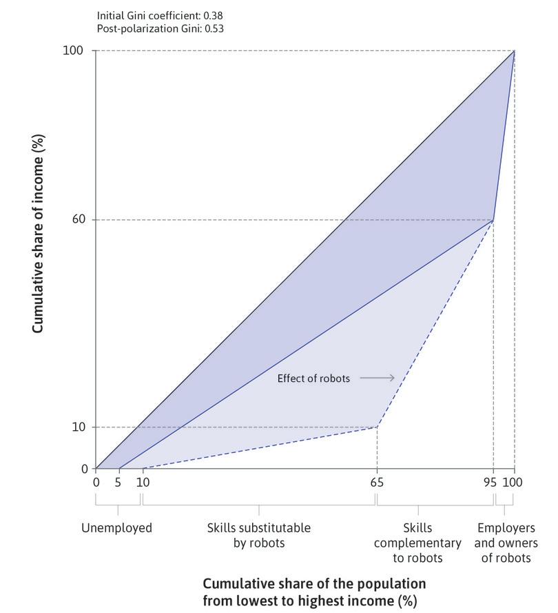
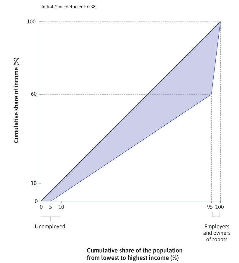
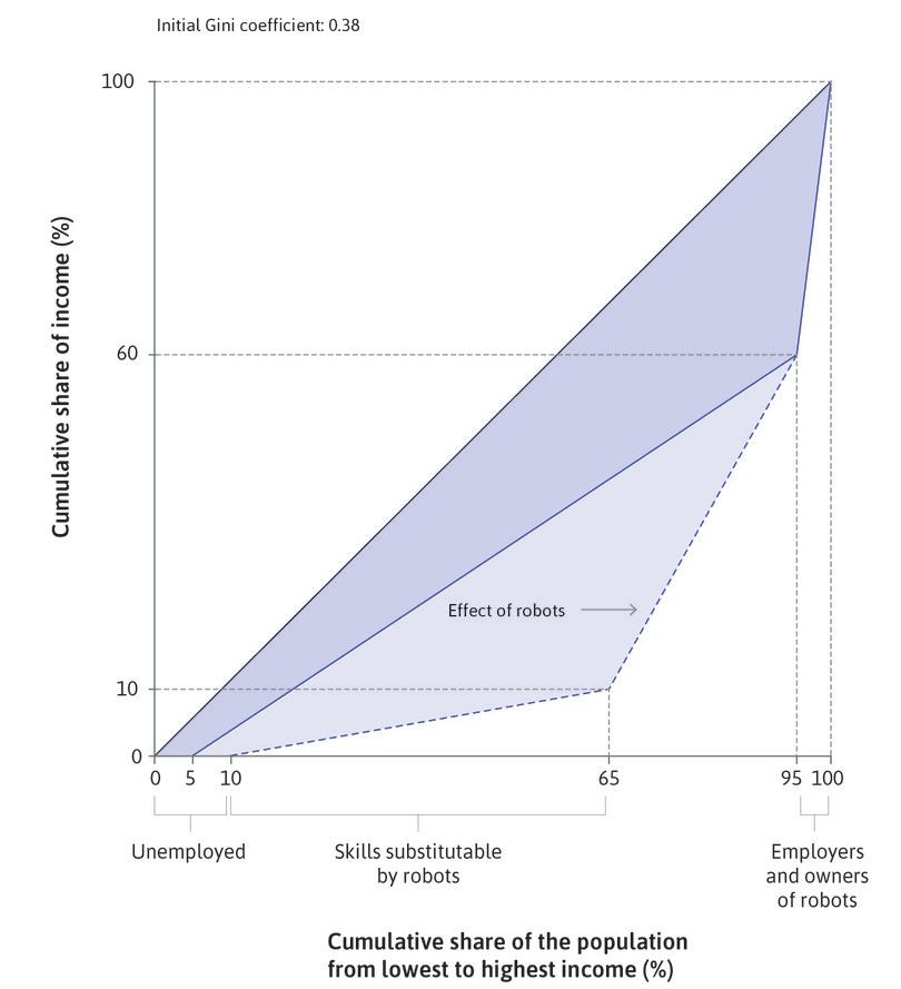
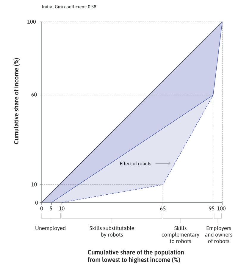
Unit 19 Economic inequality
Economic disparities are mostly a matter of where you were born, who your parents are, and (in some countries) your gender. Well-designed policies and institutions can reduce inequalities without lowering average living standards
- Having declined for most of the twentieth century, inequality of income then increased in the US, the UK, India, and many other countries.
- Nonetheless, because of the rapid economic growth of China and India, countries with very large populations, income inequality among all people in the world has declined since the end of the twentieth century.
- Discrimination based on race, gender, or religion, and other forms of unequal opportunity mean that otherwise identical people will have different incomes and economic opportunities, contributing to inequality.
- Income disparities among people are due to what they own (for example, a piece of land), are (male or female), or have (particular skills) that enable them to receive income.
- The institutions and policies in force in a society and the technologies used in production influence these determinants of income.
- Some inequalities provide incentives to study and work hard, and to take the risks associated with innovation and investment.
- But inequalities also restrict economic opportunities of the less well off and may also result in a more conflict-ridden society and impose costs, impairing economic performance.
- Well-designed and implemented government policies can limit unfair economic inequality while raising average living standards, as has been done in many countries.
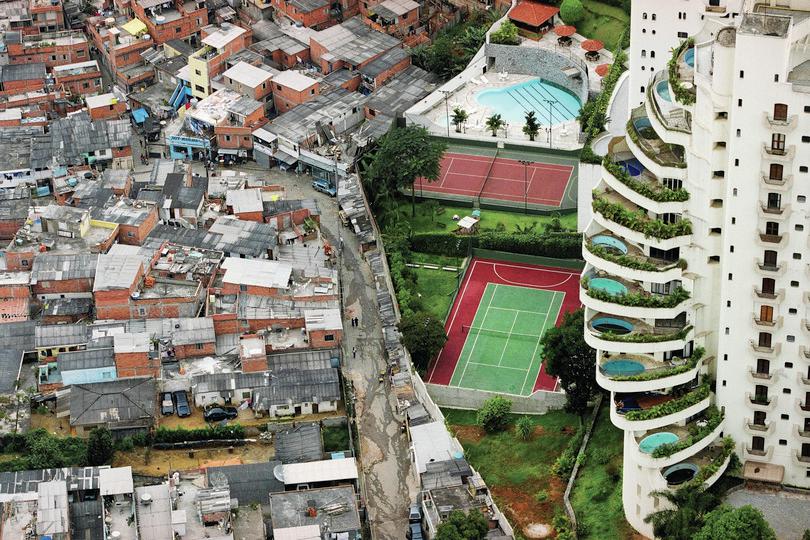
It is 1975. Renfu is the child of a local Communist Party leader. In 10 years, he will attend Tsinghua University, an elite engineering university in Beijing, and will join the Communist Party himself. In 20 years, he will run a state-owned enterprise. In 30 years, he will be CEO of the company after it is privatized, and be highly ranked within the Party.
However, Yichen, whose parents have no party connections, will not go to university, but instead work the land alongside her parents until she is 16, and then work at a state-owned enterprise making car parts for export to the US and Europe. When she is 30 years old, she will take a job in the new Motorola factory opening in nearby Tianjin, paying double her current wage. She will not be able to migrate legally to Tianjin and leaves her daughter behind with her parents.
Yichen and Renfu are hypothetical people. We could have inserted a disclaimer: ‘All characters appearing in this work are fictitious…’ But that would not be entirely true—they illustrate the divergent histories of real people alive today.
Let’s also consider two other hypothetical people living in the US, also in 1975. Mark and Stephanie, both 17, live in Gary, Indiana. Mark is about to finish high school and start working in the local unionized steel mill with his father, where the pay is good and he doesn’t have to spend four years in further education before earning a wage.
In the 1981 recession, Mark will lose his job. He will try to use his mechanical ability to open a car parts business. With little wealth of his own to post as collateral, he will not be able to obtain a bank loan, so he will move south to another factory. This one is non-unionized, and he will make less money than he did in Gary. In 2008, during the recession, his factory will replace him with a KUKA Robotics Corporation Titan industrial robot.
Stephanie, both of whose parents are doctors, decides she will attend Indiana University Bloomington, majoring in psychology. Afterwards she will work for a large financial corporation in Chicago and, after a series of promotions, becomes a vice-president for human resources. She will invest her savings in the stock market, which yields an average return of more than 10% for many years, and will benefit from government tax cuts that favour high earners.
These four people had very different life outcomes. Is there anything wrong with that? Each of the four made good choices knowing what they could have known at the time, everybody worked hard, and yet they had very different lives. We might say that they simply drew different hands in the card game of life.
Their parents are an important difference in the hands that they drew. This starts with the fact that Yichen and Renfu were born in China, and Mark and Stephanie in the US. The parents of the two in China were likely to be equally poor, although Communist Party members enjoyed a higher level of social prestige and education. The gap in wealth between the two sets of American parents would probably have been larger. If Mark was black the gap would be greater than if he was white, but his family would still have been far better off in material terms than both the Chinese families.
In 2017, the children of Stephanie and Renfu, who have been relatively successful in each country, will have access to a variety of opportunities not available to the children of Yichen and Mark. In China, Renfu’s children will attend better schools and have better job prospects because of their father’s connections. With luck, they may attend a US university, gain valuable work experience in the university-trained, English-speaking global labour market, and return to China with salaries many times those of the average Chinese citizen.
Yichen’s daughter will not obtain a high-quality primary or secondary education. This is because the hukou restrictions mean she must go to school in Yichen’s rural home district and not in Tianjin, where her mother works. Nevertheless, most likely she will be better off over her lifetime than her parents, and will certainly be better off than her grandparents.
In the US, Stephanie’s children will attend either a public school in her expensive neighbourhood, well funded by local property taxes, or an expensive private school. They will get early access to a much larger vocabulary, form lifelong friendships with other kids from their privileged background, and engage in a variety of interesting extracurricular experiences that help their educational performance and will help them get admission to elite universities. This will translate into average lifetime earnings of close to $800,000 greater than the earnings of those whose education finishes at high school level.1
Mark’s children will have to deal with poorly funded public schools, the absence of union jobs, a minimum wage that will be worth less in real terms than it was in their parents’ generation, and changes in technology and trade that will amplify the effects of these problems. The life trajectories of these four people illustrate just a few of the global changes in the distribution of income that have occurred in the past 40 years.
Inequality exists across many dimensions, including income, wealth, education, health, and other opportunities. In this unit, we will focus primarily on inequalities in wealth and income, both because they have been studied extensively by economists and because they are strongly related to other forms of inequality. We begin with three sets of facts:2 3
- Inequality of income: In the next section, we survey evidence from around the globe about inequalities in income and how they have changed in the past century.
- Accidents of birth: We then look at inequality through an alternative lens. Accidents of birth influence one’s income, whether it be one’s nation, race, gender, wealth, or even the quality and extent of one’s schooling.
- The future of inequality: The last set of facts offers a glimpse into the future of the rich economies, looking at the kinds of jobs available as automation and the global relocation of industrial production accelerate the transition from a manufacturing to a service-producing economy.
We then ask why inequality is widely seen as a problem, and provide a way to approach the question of whether there is too much (or too little) inequality. We present a model of the causes of economic inequality in order to understand how public policies and other changes can alter the degree of economic inequality. And we then use this model to explain both recent changes in the levels of economic inequality in a number of countries, and the effects of government policies on the degree of inequality.
Exercise 19.1 Income variation across and within countries
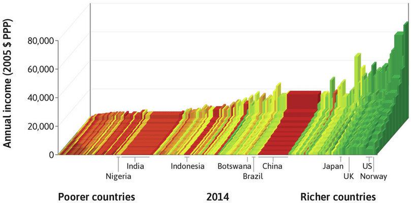
In Unit 1, Figure 1.2 showed the distribution of income across and within countries in 2014. The height of each bar in the chart varies along two axes. The first axis of variation, from left to right of the figure, is a ranking of countries according to gross domestic income per capita from the poorest on the left (Liberia), to the richest on the right (Singapore). The second axis, from the front to the back of the figure, shows the distribution of income from poor to rich within each country.
You can find an interactive version of this figure at http://tinyco.re/7434364.
Go back over the stories of Mark, Renfu, Stefanie, and Yichen and make your guess about which decile fits each of the fictional characters. Briefly justify your choice.
19.1 Inequality across the world and over time
As you know from Unit 5, we can use Lorenz curves to estimate Gini coefficients, which measure the degree of inequality in wealth, income, earnings (income from work in the form of salaries and wages), years of schooling, and other indicators of economic or social success.
Wealth, earnings, market income and disposable income
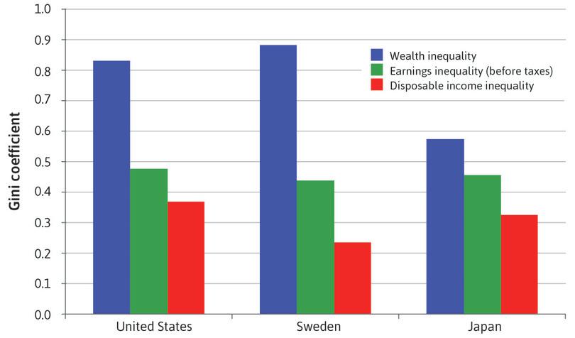
Figure 19.1 shows data on three dimensions of inequality (wealth, earnings, and disposable income) in three economies. Recall that wealth is the value of the assets owned by a household (net of their debts). Earnings are income from labour, including from wages, salaries, and self-employment. Market income is the sum of:
- all income received as earnings
- all income received from business owned by the household or from investments
Finally, disposable income is the income that a family can spend
- after paying taxes
- after receiving any monetary transfers from the government such as unemployment benefit and pensions
Two things stand out in Figure 19.1:
- Wealth is much more unequally distributed than earnings, and earnings are much more unequally distributed than disposable income: Though the differences among the three measures of inequality are much smaller in Japan than in Sweden and the US.
- Sweden has much lower disposable income inequality than the other two countries: This is due to its relatively modest inequality in earnings and more importantly, to its system of taxes and transfers which benefits the less well off. It is not due to greater equality in Sweden’s distribution of wealth. As you can see from the graph, wealth is distributed almost as unequally in Sweden as in the US.
Inequality in wealth, earnings, and disposable income: US, Sweden, and Japan (2000s).
Figure 19.1 Inequality in wealth, earnings, and disposable income: US, Sweden, and Japan (2000s).
Mattia Fochesato and Samuel Bowles. 2013. ‘Wealth Inequality from Prehistory to the Present: Data, Sources and Methods.’ Dynamics of Wealth Inequality Project, Behavioral Sciences Program, Santa Fe Institute; Mattia Fochesato and Samuel Bowles. 2017. ‘Technology, Institutions and Wealth Inequality in the Very Long Run’. Santa Fe Institute; Chen Wang and Koen Caminada. 2011. ‘Leiden Budget Incidence Fiscal Redistribution Dataset’. Version 1. Leiden Department of Economics Research.
Income inequalities over time and among countries
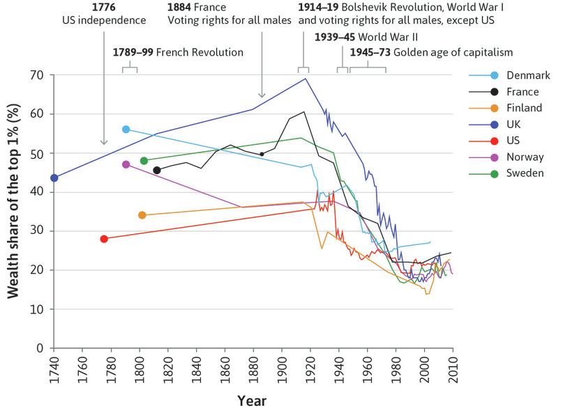
Another way to measure inequality focuses on the very rich, providing an answer to the question: what fraction of total income or wealth belongs to the richest 1% or 10% of the population? This indicator has the advantage that it can be measured over hundreds of years, because the very rich have long been required to pay taxes, and hence we have reasonably good information on their incomes and wealth. Figure 19.2 shows the fraction of all wealth held by the richest 1%, for all countries on which long-run data is available.4
Share of total wealth held by the richest 1% (1740–2011).
Figure 19.2 Share of total wealth held by the richest 1% (1740–2011).
Adapted from Figure 19 of Daniel Waldenström and Jesper Roine. 2014. ‘Long Run Trends in the Distribution of Income and Wealth’. In Handbook of Income Distribution: Volume 2a, edited by Anthony Atkinson and Francois Bourguignon. Amsterdam: North-Holland. Data.
There appear to be three distinct periods: the eighteenth and nineteenth centuries up to about 1910 show increasing wealth inequality (excepting Norway and Denmark), the twentieth century until 1980 shows decreasing wealth inequality, and the period since shows a modest increase in wealth inequality.
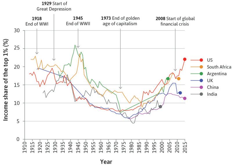
Figure 19.3 presents similar data for the share of income before taxes and transfers (rather than wealth) received by the top 1% of income earners. As in Figure 19.2 there are cross-country differences. For example, in recent years the US is much more unequal than China, India, or the UK. But there are also common trends, similar to the second and third periods in the distribution of wealth: a trend towards less inequality in much of the first three quarters of the twentieth century, followed by an increase in inequality since about 1980.
The share of total income received by the top 1% (1913–2015).
Figure 19.3 The share of total income received by the top 1% (1913–2015).
Facundo Alvaredo, Anthony B. Atkinson, Thomas Piketty, Emmanuel Saez, and Gabriel Zucman. 2016. ‘The World Wealth and Income Database (WID)’.
Explore the top incomes in countries that you are interested in the World Wealth and Income Database.
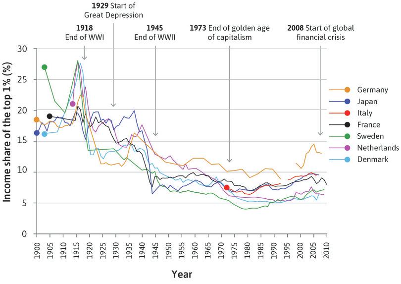
But this sharp U-turn towards greater inequality did not occur in all countries, including most of the major economies of the continent of Europe. These are shown in Figure 19.4.
Declining share of the top 1% in some European economies and Japan (1900–2013).
Figure 19.4 Declining share of the top 1% in some European economies and Japan (1900–2013).
Facundo Alvaredo, Anthony B. Atkinson, Thomas Piketty, Emmanuel Saez, and Gabriel Zucman. 2016. ‘The World Wealth and Income Database (WID)’.
Looking at Figures 19.2 to 19.4, one can see that:
- There are common trends across most of the countries for which we have data: For example, a fall in inequality between 1920 and 1980.
- Countries differ greatly in what happened since 1980: In some of the world’s largest economies—China, India, and the US—inequality rose steeply, while in others—Denmark, France, and the Netherlands—inequality remained close to historically modest levels.
We used data created by Thomas Piketty and his collaborators to create Figures 19.3 and 19.4. He is an economist and author of the bestselling economics book Capital in the Twenty-First Century.5 In our ‘Economist in action’ video, he examines economic inequality from the French Revolution to today, and explains why careful study of the facts is essential.
Inequalities between and within nations
At the beginning of Unit 1 you read that prior to the emergence of capitalism, the income a daughter or a son received depended on where their parents were on the economic ladder. It mattered much less in which part of the world the son or daughter was born.
The economic take-off of the first capitalist economies changed this.
The ‘great divergence’ in Unit 1 resulted because the kink in the hockey stick for per capita income came earlier for some countries (Britain, Italy, and Japan in Figure 1.1a), later for others (China and India), and is yet to occur for still others (Nigeria and Argentina) (see also Figure 1.11). The result of the uneven timing of the capitalist revolution around the world was a widening of inequalities among the people of the world, which occurred over the nineteenth and twentieth centuries until very recently. Even the poor in North America and Europe became richer than the rich elsewhere.
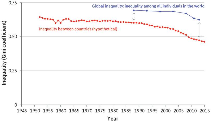
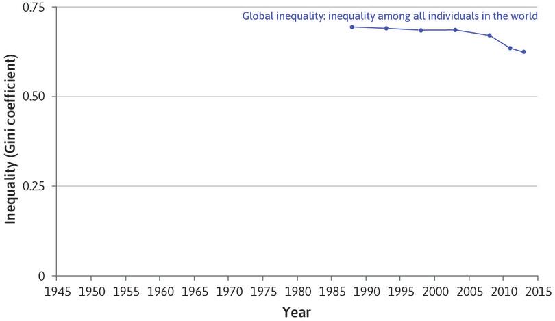
How do we measure global inequality? Think about the Lorenz curve constructed by lining up all the individuals in the world from lowest to highest income, irrespective of the country people live in. You know from Figure 1.2 that the poorest 20%—the part of the Lorenz curve extending from zero to 0.20 on the horizontal axis—would be very flat: this would represent most of the populations of Liberia and Nigeria, and middle and lower income people in Indonesia and India for example. If we construct the entire Lorenz curve, we can calculate the Gini coefficient for the whole world. This is shown for market income in Figure 19.5. For example, in 2003 the worldwide Gini coefficient was 0.69. We can see that inequality among the world’s individuals is high but has fallen very recently.
The other series in Figure 19.5 (the red line) presents global inequality in a different way. It focuses on the income differences between countries. Imagine that everyone in each country earned the average income for that country. In this thought experiment, everyone in the UK would earn exactly the UK’s average income, whereas everyone in China would earn exactly the Chinese average income. What would income inequality look like in this hypothetical example?
The red line shows the result of performing this calculation. In our thought experiment, the only source of inequality in the world would be inequality across countries. Inequality is reduced, but substantial inequalities still exist due to the vast differences in income between countries.
You can see that the Gini coefficient for all individuals in the world in 1988 (the beginning of the blue line) was 0.69, and this number would have been 0.60 had there been perfect equality within each country (the red line). As a result, we see that 87% of global inequality in income is accounted for by our measure of inequality between countries (that is because 0.60/0.69 = 0.87, or 87%).
The figure also shows that between-country inequality has been falling rapidly: by 2013, 76% of global inequality was between-country inequality (0.47/0.62 = 0.76).
The most recent Gini coefficient for the whole world is 0.62. You know that this is closer to 1 (one person has all the income in the world) than to 0 (no income differences in the world). But how much inequality does this really indicate? To see how to interpret the Gini coefficient, read the Einstein: ‘The Gini Coefficient and worldwide income differences’, which is at the end of this section.
Figure 19.5 has three main messages for us:
- Most of the inequality in the world is between individuals in different countries (the red series): It is not between individuals in the same country (the difference between the blue and red series).
- But this is changing: The world’s two largest and once very poor economies—India and China—raised their average incomes more rapidly than the richer countries, reducing between-country inequality, and because inequalities across individuals in these countries and many other large nations became greater, increasing within-country inequality.
- Inequality between individuals is declining: The net result of these opposite trends is that inequality among the individuals of the world has started to decline.
A glimpse into the future of the rich economies: The missing middle?
The increased inequality that has occurred within many developed countries has been associated with a changing distribution of jobs. Low-paying jobs and high-paying jobs have increased in number while middle-income jobs have become scarcer. The result—more jobs at the top and the bottom of the economic ladder, and fewer on the middle rungs—has been termed ‘the missing middle’.
The data in Figure 19.6 illustrate both trends for the US economy. We have used the US economy as an illustration because of the quality of the available data, but similar trends are evident in other high-income countries.
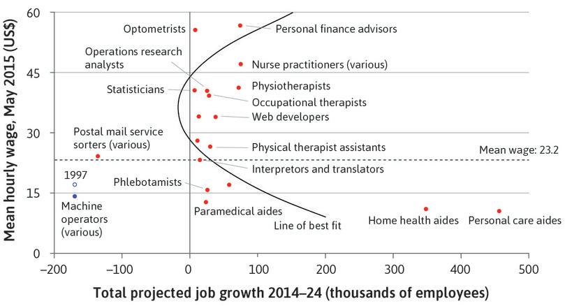
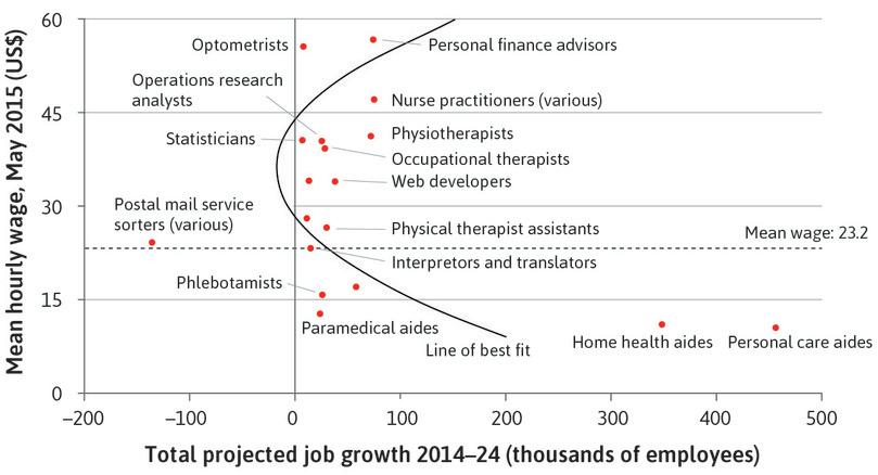
Figure 19.6 arranges jobs from the highest paid (in hourly wages) at the top to the lowest paid jobs at the bottom, and estimates growth or contraction of employment on the horizontal axis.
Note: Figure 19.6 shows only the occupations that are projected to undergo changes of 10,000 employees or more. The term ‘various’ indicates similar occupations. The blue dots are the occupations related to machine operators (sewing machine operators, textile machine operators, switchboard operators, machine operators, and molding). The horizontal dashed line is the average hourly wage across all occupations in the US in June 2015. The C-shaped line is a second-order polynomial that fits the data shown in the chart.
The dot labelled ‘1997’ shows the mean hourly wage machine operators would have earned in 2015 had their wage remained in the same proportion to the mean wage as in 1997.
Notice these things about the data:
- The missing middle: Both high-wage and (especially) low-wage occupations are adding many jobs, but employment gains among the occupations with wages in between are more limited.
- Jobs replace work once done by family members: The biggest increases are in human services, most of them in health-related professions. These growing occupations substitute for work once done primarily by family members, such as personal care aides and home health care aides.
- Machines do routine work: Digitalization reduces the demand for jobs that involve routine tasks, such as postal mail sorters and machine operators. The tasks that machines are not replacing tend to be either well paid (personal financial advisors, nurse practitioners) or poorly paid, such as those taking care of the elderly at home.
- High-wage job gainers work with information technologies: Growing occupations with high wages (outside human services) such as operations researchers, statisticians, and web developers are those in which digital information processing has greatly increased the productivity of workers with the right kinds of skills.
- Workers with average wages are the losers: Occupations with job losses tend to have near-average wages or less.
Figure 19.6 only showed occupations for which gains or losses are projected to be at least 20% of their 2014 level and change by at least 10,000 employees. But as Figure 19.7 shows, this pattern holds when we look at all jobs in the US economy. The projected trends shown in Figures 19.6 and 19.7 have been underway in the US since at least the 1970s.
The missing middle in the US (2014–24): Job growth is highest in the top fifth and bottom fifth of occupations in the US, by mean annual earnings.
Figure 19.7 The missing middle in the US (2014–24): Job growth is highest in the top fifth and bottom fifth of occupations in the US, by mean annual earnings.
US Bureau of Labor Statistics. 2014. ‘Employment Projections’. US Bureau of Labor Statistics. 2015. ‘Occupational Employment Statistics’.
Exercise 19.2 Inequalities among your classmates
- Using this Gini coefficient calculator, calculate the degree of inequality of height among your classmates.
- Why is this Gini coefficient so much smaller than it was for wealth in Figure 19.1?
- Now use the calculator to compute the Gini coefficient for another measure (for example, age, weight, commuting time to university, number of siblings, or grade in the last exam).
- Explain any differences between this Gini coefficient and that for wealth.
Question 19.1 Choose the correct answer(s)
Figure 19.1 shows the inequality in wealth, earnings, and disposable income in the US, Sweden, and Japan using the Gini coefficient.
Based on this information, which of the following statements are correct?
- In all three countries, the Gini coefficient for wealth is higher than the Gini coefficients for earnings, indicating higher inequality.
- Sweden is more unequal than Japan in terms of wealth, but is more equal in terms of disposable income.
- This statement is true for earnings and disposable income. However, Sweden is more unequal than the US in terms of wealth.
- While the Gini coefficient for Sweden’s before-tax earnings is similar to that of the US and Japan, the Gini coefficient for disposable income is much lower, indicating that taxes and transfers were effective in redistributing income.
Question 19.2 Choose the correct answer(s)
In Thomas Piketty’s ‘Economist in action’ video, which of the following were NOT among the reasons that Piketty gave for the fall in the incomes of the very rich during the twentieth century?
- Nationalization of assets during the World Wars is one of the reasons Piketty gives.
- Economic recession is one of the reasons Piketty gives.
- Although political change can affect the distribution of wealth in a country, Piketty does not mention the Russian Revolution in the video.
- Nationalization of assets during the World Wars is one of the reasons Piketty gives.
Question 19.3 Choose the correct answer(s)
Figure 19.6 is a scatterplot of occupations for the US economy, with the 2015 mean hourly wages on the vertical axis and the 2014–24 projected job growth on the horizontal axis:
Based on this information, which of the following statements is correct?
- Occupations with the biggest projected growth are home health aides and personal care aides. These are services that were once produced almost exclusively in the family but are now being increasingly performed by employees outside the home.
- Occupations with substantial projected job losses are those near average wages or less that are already affected by technologies that allow human replacement, such as postal mail service and switchboard operators.
- The biggest increases are in human services, most of them in health-related professions. High-wage jobs that involve information technologies are also projected to grow.
- Both high- and low-wage occupations are projected to add jobs, while those in between seem to have limited prospects of employment gains.
Einstein The Gini coefficient and worldwide income differences
In Unit 5 you learned that the Gini coefficient is a measure of inequality that is defined as half of the relative mean differences in incomes between all pairs of people in a population.
Recall that the mean difference in incomes among all pairs in the population which we denote as Δ can be expressed as the income of the richer of the pair (yr) minus the income of the poorer of the pair (yp) summed over all of the pairs in the population, and then divided by the number of pairs in the population (n). The relative mean difference is this quantity divided by mean income, y.
So half of the relative mean difference is:
By rearranging this equation, you can see that the average difference between the two paired people will be the mean income times twice the Gini coefficient:
But there is a more interesting interpretation of the Gini coefficient. If we have drawn all possible pairs from the world’s population, the mean income in the world () will be:
where we defined and are the average incomes of the richer and the poorer of each of the pairs, respectively. So we can now rewrite the expression for the Gini coefficient in terms of and :
By rearranging and dividing through by , we have:
Using this final expression, if the Gini coefficient for the world is 0.62, then:
This says that if the Gini coefficient is 0.62, then across all of the pairs in the population or across a large random sample of the population, the better off of the two is on average 4.26 times richer than the less well off.
Exercise 19.3 Another way to interpret Gini coefficients
Use Figure 5.16 to estimate the Gini coefficient for disposable income in Denmark and South Africa. In explaining the difference in income inequality between these two countries, you could use the information in the Gini as follows: if two people are chosen at random from the population of the country, what is the average ratio of the richer person’s income to that of the poorer person’s? To allow you to translate data on the Gini coefficient into this ratio, use the formula in the Einstein to construct a table of the richer/poorer ratio for Gini coefficients ranging from 0.0 to 0.9 (in increments of 0.1). Graph your results. Explain the difference in inequality between Denmark and South Africa using your results. What does the formula imply if the Gini coefficient is equal to 1?
19.2. Accidents of birth: Another lens to study inequality
Much of the inequality in the world today can be traced to differences among people in things over which they have virtually no control, such as their race, sex, nation, or parents. We call these differences ‘accidents of birth’.6
To see how important accidents of birth can be, try the following thought experiment. Go back to Figure 1.2. Suppose that all you care about is income, and you can choose either:
- the income decile you are in, but the country you are born in will be decided by chance
- the country you are born in, but the decile you are in within the country will be decided by chance
Did you choose option 1 (the decile) or option 2 (the country)?
If you chose option 1, you would of course choose to be in the top decile, so you would be somewhere at the back of Figure 1.2. But where? You would have an equal chance of being born in Nigeria on the left-hand side or in the UK on the right-hand side.
If you chose option 2, you could select one of countries at the right-hand end with the highest average income. You are as likely to be in the lowest decile, at the front of the figure, as in the highest decile, at the back.
One’s citizenship is one of the great accidents of birth affecting income. Passports and borders limit the economic opportunities people from different countries face. People with the same education, capacities, and ambition but born on different sides of a national border face very different life chances, whether that is the border between Mexico and the US, The People’s Democratic Republic of Korea (North Korea) and South Korea, or the Mediterranean Sea that divides North Africa from Europe. Even where migration is allowed, migrants are often denied access to political and labour rights, as in the Gulf States and some East Asian countries.
Gender and other forms of categorical inequality
Inequalities based on accidents of birth also exist within countries:
- Caste: Vast disparities in life chances in India, for example, follow from long-established hereditary and hierarchical ‘caste’ boundaries. Caste is a social status that ranges from high-status Brahmins to Dalits (once called ‘untouchables’).
- Formalized discrimination: Until 1994, apartheid in South Africa formalized inequality with a complex system of racial barriers.
- Colonists and indigenous people: In Australia, the US, and much of Latin America, extraordinary economic and social inequality exists between descendants of European colonists and those who arrived tens of thousands of years earlier, called indigenous people.
- categorical inequality
- Inequality between particular social groups (identified, for instance, by a category such as race, nation, caste, gender or religion). Also known as: group inequality.
Inequalities based on one’s ethnic identity or caste are examples of categorical inequality (also known as group inequality), meaning economic differences among people who are treated as being in different social categories as defined by more powerful social classes. The Indian castes are categories, as are those of ‘African’, ‘White’, ‘Coloured’ and ‘Asian’ in South Africa. Categorical inequalities are for the most part based on accidents of birth, because one is born into membership in one of the categories, and switching category is typically difficult if not impossible.
To understand how easily segregation by race or some other categorical characteristic arises, take two minutes to play the online game The Parable of the Polygons.
The most common form of categorical inequality is that between men and women. There are many economic differences between men and women on average. This is a bit puzzling because other than differing biological roles in reproduction, men and women are so similar: similar parents, similar schools (in most countries), similar genetic inheritance on matters affecting intellectual skills and so on. But it is clear that the economy treats men and women differently. This is much more true in some countries than in others, but it is true for all countries.
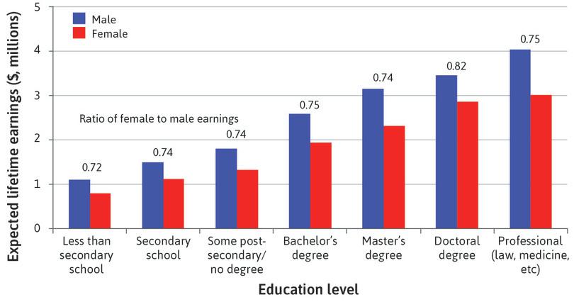
Income disparities between men and women among otherwise similar individuals are one measure of this inequality. Figure 19.8 shows the expected lifetime earnings (labour income) of men and women in the US, who work full time from the time they leave school until retirement. As a result, any differences in the figure are not due to women having more time out of the labour force (on average) because of child rearing.
Because the quality of schooling does not differ between males and females on average (and girls tend to do as well on most tests), the gender differences in pay are not due to differences in cognitive ability or quality of schooling. Yet for every level of schooling, women can expect to earn much less than men.
Categorical inequality: Schooling and lifetime earnings for men and women in the US.
Figure 19.8 Categorical inequality: Schooling and lifetime earnings for men and women in the US.
Adapted from Figure 5 in Anthony P. Carnevale, Stephen J. Rose, and Ban Cheah. 2011. The College Payoff. Georgetown University Center on Education and the Workforce. (Note: The average for males is $2,520,286, while for females it is $1,909,714.)
The figure also shows, however, that additional schooling contributes to higher lifetime incomes, and that those women who complete university (a bachelor’s degree) can expect to earn much more than men who ended their schooling after secondary school.
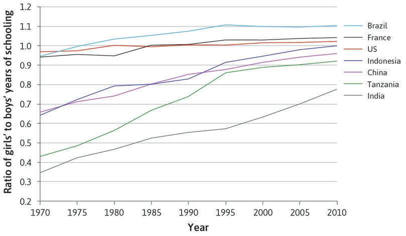
In many parts of the world girls receive considerably less schooling than boys, but as Figure 19.9 shows, girls go to school for the same number of years on average as boys in both the US and France, and longer in Brazil. Countries in which women have historically suffered extraordinary social and economic disadvantages, such as China and Indonesia, have virtually eliminated the gender gap in years of schooling, and India, though far behind, is rapidly closing it.
Categorical inequality: Average years of schooling, girls relative to boys (1970–2010).
Figure 19.9 Categorical inequality: Average years of schooling, girls relative to boys (1970–2010).
The World Bank. 2016. IIASA/VID Educational Attainment Model. Dataset produced by the International Institute for Applied Systems Analysis (IIASA) in Luxemburg, Austria and the Vienna Institute of Demography, Austrian Academy of Sciences. Educational Attainment Statistics.
Intergenerational inequality
In addition to categorical differences such as nation, gender, race, or ethnic group, a second source of economic inequality within a nation is inherited. You may be rich or poor simply because your parents were rich or poor.
Two hundred years ago, in most countries it was taken for granted that somebody would expect a life of poverty simply because her parents had been poor, or that someone else would inherit the ownership of his father’s company and social status, without having to prove that he was the best person for the job. The inheritance of inequality from one generation to the next seemed to be part of the natural order of things.
But this has changed with the spread of public education and, in many countries, with the decline in discrimination against poor people due to their race, religion, or simply their humble origins. In some countries, the economic status of one’s parents matters a great deal for the economic success of their children; in other countries, differences among parents are only weakly transmitted to their offspring.
- intergenerational transmission of economic differences
- The processes by which the economic status of the adult sons and daughters comes to resemble the economic status of the parents. See also: intergenerational elasticity, intergenerational mobility.
The expression intergenerational transmission of economic differences refers to the processes by which the economic status of the adult sons and daughters comes to resemble the economic status of the parents. The transmission process takes many forms:
- Children inherit the wealth of their parents.
- The genetic makeup of the children is similar to the parents.
- Through parental influence in child rearing, parents and children tend to share similar preferences, social norms, and knowledge, skills and social connections acquired outside formal schooling.
- intergenerational inequality
- The extent to which differences in parental generations are passed on to the next generation, as measured by the intergenerational elasticity or the intergenerational correlation. See also: intergenerational elasticity, intergenerational mobility, intergenerational transmission of economic differences.
Intergenerational inequality occurs where these processes result in similarity between the economic status of parents and their children: the children of the well off become rich themselves, while the children of the less well off stay poor.7
Economists and sociologists measure intergenerational inequality by ranking parents by their incomes or wealth, and then looking at what income or wealth their kids end up with when they become adults. They confirm that there is substantial intergenerational inequality. Kids whose parents had a high income are likely to grow up to have high incomes themselves, and kids from low-income families are likely to have low incomes as adults.8
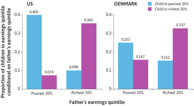
This is what we see in Figure 19.10, which gives measures of the intergenerational inequality of men in the US (left panel) and Denmark (the right panel), based on their labour earnings (wages or salaries). The tall bar on the left in the US panel means that among those whose fathers were in the bottom fifth of the earnings distribution, 40% were themselves in the poorest fifth, while 7% ended up in the top fifth of the earnings distribution. By contrast, 36% of those born to the richest fifth were themselves in the richest fifth—the tall purple bar on the right.
Intergenerational inequality in earnings: The US and Denmark.
Figure 19.10 Intergenerational inequality in earnings: The US and Denmark.
Table 14 in Markus Jäntti, Bernt Bratsberg, Knut Røed, Oddbjørn Raaum, Robin Naylor, Eva Österbacka, Anders Björklund, and Tor Eriksson. 2006. ‘American Exceptionalism in a New Light: A Comparison of Intergenerational Earnings Mobility in the Nordic Countries, the United Kingdom and the United States.’ Discussion Paper Series 1938. Institute for the Study of Labor.
One of the reasons that children of the rich tend to be richer than the children of the poor is the financial support that rich parents give to their children, both during the parents’ lifetimes and at death in the form of inheritances. The data in Figure 19.10, however, is based on labour earnings, not inherited wealth. The earnings of parents and their children appear to be similar in the US, partly because children of well off parents receive more, higher-quality, schooling. They also benefit from the networks and connections of their parents, which improve access to the labour market.
The data from Denmark in the right panel suggests a more level playing field. Only 25% of those born to parents in the poorest fifth of the population end up in the poorest fifth themselves, compared to 40% in the US. This suggests that those born to relatively poor parents are less disadvantaged in Denmark. Similarly, 33% of those born to parents in the richest fifth end up in the richest fifth themselves, compared to 36% in the US. Based on this data, we would conclude that intergenerational inequality is lower in Denmark than in the US, though it still does not appear to be a completely level playing field.
- intergenerational elasticity
- When comparing parents and grown offspring, the percentage difference in the second generation’s status that is associated with a 1% difference in the adult generation’s status. See also: intergenerational inequality, intergenerational mobility, intergenerational transmission of economic differences.
A measure that can summarize the overall rate of intergenerational inequality in a society is the intergenerational elasticity of income or wealth. To see what this measures, consider two pairs of fathers and children. The father in the first pair is richer than the father in the second. The intergenerational elasticity measures how much richer the child of the well off father will be than the child of the poorer father. An elasticity of 0.5, for example, means that if one father is 10% richer, then his child, when grown up, will be on average 5% richer than the other child. The higher the intergenerational elasticity, the greater the degree of intergenerational transmission of economic status and the greater the level of intergenerational inequality. In a society with a high intergenerational elasticity, intergenerational mobility is low.
The term intergenerational elasticity has nothing to do with the usual meaning of the word elastic. But, like the price elasticity of demand for a good, it concerns the percentage change in something that is associated with a percentage change in something else.
- intergenerational mobility
- Changes in the relative economic or social status between parents and children. Upward mobility occurs when the status of a child surpasses that of the parents. Downward mobility is the converse. A widely used measure of intergenerational mobility is the correlation between the positions of parents and children (for example, in their years of schooling or income). Another is the intergenerational elasticity. See also: intergenerational elasticity, intergenerational transmission of economic differences.
What is the relationship between a measure of intergenerational inequality such as the intergenerational elasticity and the extent of inequality among the members of a population at a given point in time? You can think of many reasons why the two would go together.
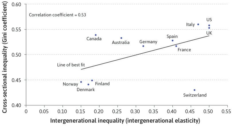
Figure 19.11 presents evidence on the relationship between intergenerational elasticity for earnings and earnings inequality at a particular time. We refer to earnings inequality at a particular time, which we measure using the Gini coefficient for income, as cross-sectional inequality. Note that we do not include the effects of taxes and government transfers in Figure 19.11 when we measure both income inequality and intergenerational transmission of earnings, because we are interested in the movements of these two dimensions of inequality that are independent of government policy.
Intergenerational and cross-sectional inequality.
Figure 19.11 Intergenerational and cross-sectional inequality.
Miles Corak. 2013. ‘Inequality from Generation to Generation: The United States in Comparison.’ In The Economics of Inequality, Poverty, and Discrimination in the 21st Century, edited by Robert S. Rycroft. Santa Barbara, CA: Greenwood Pub Group; Wen-Hao Chen, Michael Förster, and Ana Llena-Nozal. 2013. ‘Globalisation, Technological Progress and Changes in Regulations and Institutions: Which Impact on the Rise of Earnings Inequality in OECD Countries?’. Working Paper Series 597. LIS.
The figure shows that for the countries considered, inequality in earnings at any particular point in time tends to be higher when intergenerational inequality is high. The US, UK, and Italy are examples of countries that have both high cross-sectional inequality and high intergenerational inequality. In other countries (Norway, Denmark, Finland) both intergenerational inequality and cross-sectional inequality are quite limited. But some countries differ according to which type of inequality is most pronounced. Compare, for example, Canada and Switzerland.
Does cross-sectional inequality cause intergenerational inequality, or the other way around, or both, or neither? We know that societies with a strong culture of fairness and equal treatment, such as Denmark, adopt policies to reduce inequality between people at a given moment, including offering generous benefits to unemployed and retired individuals through the welfare state. At the same time, they also attempt to limit intergenerational inequality by providing equal opportunities for high-quality education, and through other policies that would reduce intergenerational transmission of economic status. This is part of the explanation of the contrast between Denmark and the US in Figure 19.10.
Another likely source of the correlation in Figure 19.11 is that in any period (a generation for example), some individuals experience good luck—for example, living in a region that experienced an economic boom, while others experience bad luck—serious illness (their own or a family member), unplanned pregnancy, business failure, or because technological change or shifts in demand make their skills less valuable. These ‘shocks’ create more inequality in any given generation.
But if having high-income parents gives their sons and daughters economic advantages when they grow up, then these shocks live on even after the parents pass away. A person’s father may have been rich just by good fortune, but his son and daughter will also be rich (or at least richer than they would have been) by inheritance.
Thus, in countries where intergenerational inequality is substantial, for example in the US, Italy, and the UK, high or low incomes resulting from good luck or bad luck are passed on to the next generation, and added to whatever shocks of good or bad fortune that the next generation experiences. As a result, intergenerational inequality contributes to cross-sectional inequality.
You now know some basic facts about inequalities around the world. Knowing these facts, we ask what, if anything, is wrong with economic inequality?
Exercise 19.4 How inequalities of birth persist between generations
- Go back to the stories of Yichen, Renfu, Stephanie, and Mark and indicate all of the accidents of birth that affected their economic successes or failures.
- Give some reasons why the intergenerational inequality and inequality between members of a population at a given moment in time are positively correlated.
Question 19.4 Choose the correct answer(s)
Figure 19.10 shows the proportion of children in earnings quantile conditional on their father’s earnings quantile in the US and Denmark, respectively.
Based on this information, which of the following statements is correct?
- The intergenerational elasticity is higher for the US than for Denmark, which does not support the claim in the ideal of the American Dream.
- The purple bar at the top-left of the figure (left panel) shows this information.
- The percentage of the richest 20% fathers whose children also ended up in the richest 20% are comparable in Denmark and the US: 33.7% compared to 36%.
- The diagrams show that in Denmark, the advantage of being born in a rich family is relatively smaller and the disadvantage of being born poor is certainly smaller than in the US. This may be attributed to Denmark’s attempt to improve intergenerational mobility by, for example, providing equal opportunities for high-quality education and reducing the importance of inherited wealth.
19.3 What (if anything) is wrong with inequality?
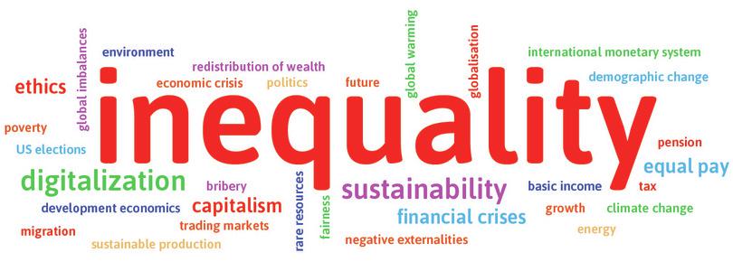
In November 2016, we asked students beginning economics at Humboldt University in Berlin, ‘What is the most pressing issue that economists today should address?’ Their replies are shown in the word cloud in Figure 19.12, in which the size of the word or phrase indicates the frequency with which that term was mentioned. Students in other universities around the world gave similar answers.
Perceived, ideal and actual inequalities
One of the reasons why inequality is seen as a problem is that many people think there is too much of it.
Michael Norton, a professor of business administration, and Daniel Ariely, a psychologist and behavioural economist, asked a large sample of Americans how they thought the wealth of the US should be distributed: what fraction of it, for example, should go to the wealthiest 20%? They also asked them to estimate what they thought the distribution of wealth actually was.9
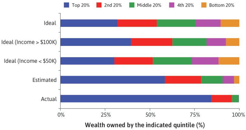
Figure 19.13 gives the results, with the top three bars showing the distribution that different groups of respondents considered would be ideal, and the fourth bar the wealth distribution that they thought actually existed in the US. The top bar shows that Americans thought that, ideally, the richest 20% should own a little more than 30% of total wealth—some inequality was desirable, but not a lot. Now contrast this with the fourth bar (‘Estimated’), which shows that they thought that the richest 20% owned about 60% of the wealth. The bottom bar shows the actual distribution. In reality, the richest fifth owns 85% of the wealth. The actual distribution is much more unequal than the public’s estimate—and contrasts sharply with the lower inequality that people would like to see.
Ideal, estimated, and actual distribution of wealth for people in the US.
Figure 19.13 Ideal, estimated, and actual distribution of wealth for people in the US.
Adapted from Figures 2 and 3 in Michael I. Norton and Daniel Ariely. 2011. ‘Building a Better America—One Wealth Quintile at a Time’. Perspectives on Psychological Science 6 (1): pp. 9–12.
Different groups largely agree on the ideal distribution of wealth. Americans with an annual income greater than $100,000 thought that the share going to the top 20% should be slightly larger than those who earned less than $50,000 thought it should be. Not shown in the figure: Democratic Party voters wished for a more equal distribution than Republican Party voters, and women preferred more equality than did men. The differences between these groups, however, were small.
When is inequality unfair?
Although there seems to be a consensus on the ideal outcome in the US, policies that would redistribute income and wealth are controversial and debated passionately—as they are in most countries. Differences in self-interest contribute to the arguments. Richer Americans, for example, tend to oppose redistribution that favours the poor, while poorer Americans support it.
But, as the experiments in Unit 4 would lead us to expect, self-interest is just part of the explanation. People differ also because they hold different beliefs about why the poor are poor and how the rich became rich. In laboratory settings, people often express strong feelings of fairness, and give up considerable sums of money to ensure that outcomes are consistent with ideas of economic justice.
For example, Responders in the ultimatum game reject what they consider an unfair offer, preferring to receive nothing and to impose the same fate on the Proposer than to agree to being treated unfairly. Both rich and poor may think that high levels of inequality are unfair and that the government should reduce economic disparities, even if it means voting for policies that would reduce the disposable income of the voter.
In Unit 5, you read about contrasting ideas about fairness, not based on how people play in experimental games, but instead on moral principles. Procedural theories, which are ideas of fairness based on how the inequality came to be, focus not on how poor or rich someone is, but instead on why the person is poor or rich.
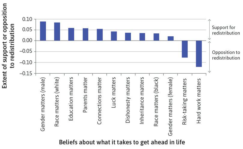
Christina Fong, an economist, wanted to know if people in the US think this way when it comes to their political support or opposition to policies to raise the incomes of the poor, financed by general taxation. She found that a person who thinks that hard work and risk-taking are essential to economic success is much less likely to support redistribution to the poor than one who thinks that the key to success is inheritance, being white, your connections, or who your parents are.
The results of her study are in Figure 19.14. Notice that white people who think that being white is important to getting ahead strongly support redistribution to the poor—evidently because they think that the process that determines economic success is unfair.
How beliefs about what it takes to get ahead predict whether people in the US support or oppose government programs to redistribute income to the poor.
Figure 19.14 How beliefs about what it takes to get ahead predict whether people in the US support or oppose government programs to redistribute income to the poor.
Figure 5.3 in Samuel Bowles. 2012. The New Economics of Inequality and Redistribution. Cambridge: Cambridge University Press; Christina Fong, Samuel Bowles, and Herbert Gintis. 2005. ‘Strong Reciprocity and the Welfare State’. In Handbook of Giving, Reciprocity and Altruism. Edited by Serge-Christophe Kolm and Jean Mercier Ythier. Amsterdam: Elsevier.
This suggests that for many people, the question ‘how much inequality is too much?’ cannot be answered unless we know why a family or person is rich or poor. Many people think it is unfair if income depends substantially on what we call an ‘accident of birth’ (categorical inequality)—your race, your sex, or your country. Inequalities based on hard work or taking risks are less likely to be seen as a problem.
Exercise 19.5 Estimated, ideal, and actual distributions of wealth
Use this Gini coefficient calculator to determine the Gini coefficients for wealth ownership given by the estimated, ideal, and actual distributions in Figure 19.13. Note: You will have to estimate the data visually from the chart.
Exercise 19.6 A level playing field
When people think about ‘too much inequality’, some think about the Gini coefficient measuring inequality at a point in time, while others are more interested in intergenerational inequality.
- Use an example of two fictional families in each country to explain the combination of cross-sectional and intergenerational income inequality in Canada and Switzerland shown in Figure 19.11.
Now think about the indifference curves that you could draw in this figure that would indicate the combinations of inequality and intergenerational inequality that would be equally fair in your judgement.
- If you cared only about the Gini coefficient and you disliked inequality, what would they look like?
- If you cared only about the intergenerational elasticity and you disliked inequality, what would your indifference curves look like?
- On Figure 19.11, draw indifference curves according to your personal preferences for cross-sectional and intergenerational inequality. Use your indifference curves to rank the countries from the fairest to the least fair.
19.4 How much inequality is too much (or too little)?
We know that accidents of birth matter. But even if the playing field were level (that is, accidents of birth did not matter), we would still face a question: how rich should the winners be compared to the losers?
A lens for looking at unfairness: The veil of ignorance.
To think about this question, transport yourself to a hypothetical world in which you (perhaps along with other fellow citizens) are asked to design your model society. There will be two groups or classes of equal size, one called ‘richer’ and the other ‘poorer’. You will get to live in the society you design after you have answered the question ‘how rich should the richer class be and how poor should the poorer class be?’
But there is a hitch: which class you get to be in will be determined by the flip of a coin after you have decided how unequal the society will be.
This thought experiment is what the American philosopher John Rawls, whom we encountered in Unit 5, termed choosing a social contract from behind a veil of ignorance. The ‘veil of ignorance’ ensures that we do not know which position we would occupy in the society we were designing.
Behind the curious device of the veil is an important concept. Rawls’ fundamental idea is that justice should be impartial. It should not favour one group over another, and the veil of ignorance invites you to think this way (because you do not yet know which group you are going to be in). Rawls asked us to think about justice as if:
[N]o one knows his place in society, his class position or social status; nor does he know his fortune in the distribution of natural assets and abilities, his intelligence and strength, and the like. (A Theory of Justice, 1971)
This does not tell us the answer to how much inequality there should be, but it does suggest a way to look at it.
Feasible inequality
Economics gives us tools for studying what combinations of the income of the rich and the poor are feasible, and how we might reason about which ones are preferable to others.
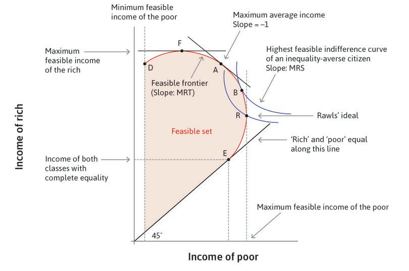
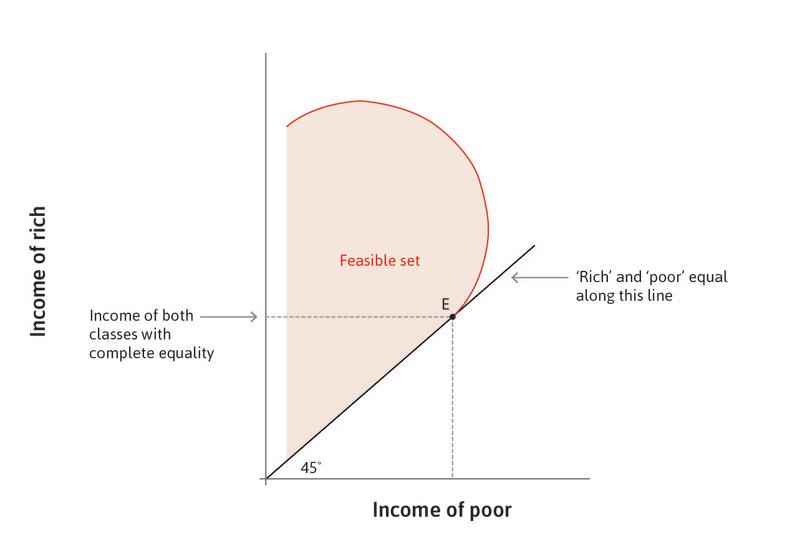
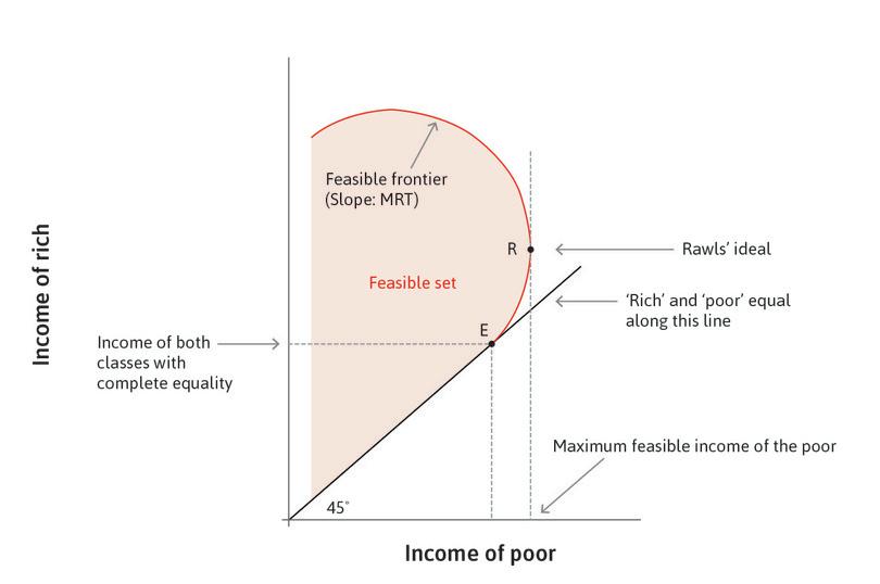
Let’s try one way to answer the question of ‘how rich should the richer class be and how poor should the poorer class be’. Let’s say there should be no difference between the incomes of the rich and the poor. Suppose that, in this case, both classes would receive $100,000 annually (per adult). This is shown by point E (for Equality) in Figure 19.15, where the 45-degree line gives all of the points of equal income between the two classes (so there is really no meaning to ‘rich’ and ‘poor’). The figure shows the annual income per adult of the poor and the rich on separate axes.
Would this be your choice? In this version of an ideal society, you would not run the risk of ending up poorer than others after the coin flip. But as an economist you might think that complete equality in the society would mean that there were insufficient incentives for people to work, study, and take risks innovating and investing, so that at least some inequality could actually be better for everyone.
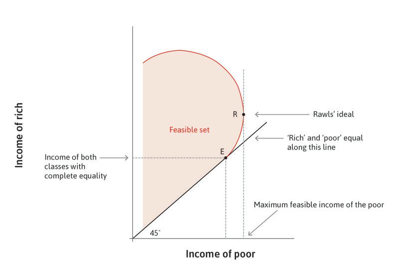
In the figure, points between E and R show possible combinations in which the rich are richer than the poor, but where the poor also are richer than they would be under complete equality. To put it another way, from any one of these points, including point E, there is a win-win possibility: giving more income to the rich allows the poor to have more income as well.
Comparing the two points, you can see that E is Pareto inefficient because both the rich and poor are better off at R than at E. The income distribution at R is also the one at which the poor are as rich as they can possibly be in this economy, as indicated by the feasible frontier. This is the point that Rawls favoured (and why we called it point R).
Would you choose R? Notice that, above R, the frontier is very steep. This means that it’s possible to make the rich much richer by making a small reduction in the income of the poor.
The red curved line passing through R and E (and the other points above R) is the frontier of the feasible set of income distributions for the economy in question. We assume that a government can adopt policies to bring about any one of these economically feasible points, but in Unit 22 we will introduce limits on the government’s ability to do so, which would have the effect of shrinking the feasible set. As with all feasible frontiers, the slope is a marginal rate of transformation. In this case, the transformation is of income losses of the poor into income gains for the rich.
If the point R had been proposed, would you want to consider other points higher up on the feasible frontier? Remember, after the coin flip, you will get either the income of the rich or that of the poor with equal probability (one half), so you know that:
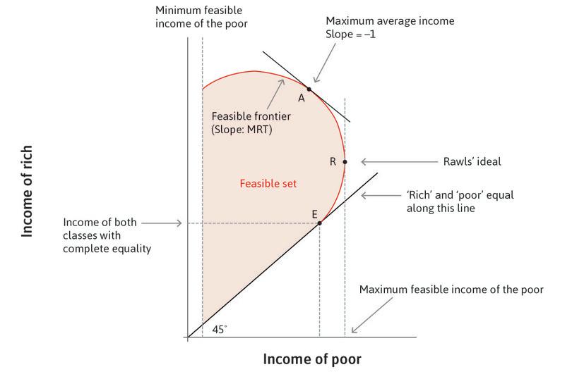
As long as income gains for the rich come at little expense of income losses for the poor, you would definitely do better to move above point R. If you were interested in maximizing your expected income and did not care about the degree of inequality, then you would choose point A, where the income gains of the rich are exactly offset by income losses by the poor, so the marginal rate of transformation is equal to one.
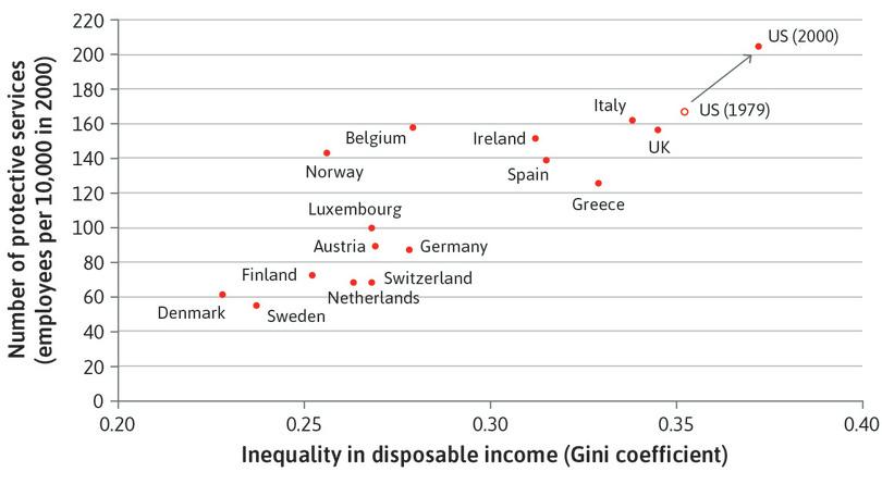
But after point A, the inequalities would become so severe that the average income would fall, and the rich would be getting a larger slice of a smaller pie. This might occur if the poor were not fed enough to work hard, or were angry enough about their condition to motivate the rich to divert some economic resources from goods and services production into protecting their wealth, which reduces total output. By looking ahead to Figure 19.30c, you will see data showing that more unequal societies (such as the US, UK, and Italy) devote more resources to workers employed in private and public security activities than do other more equal countries with similar GDP per capita.
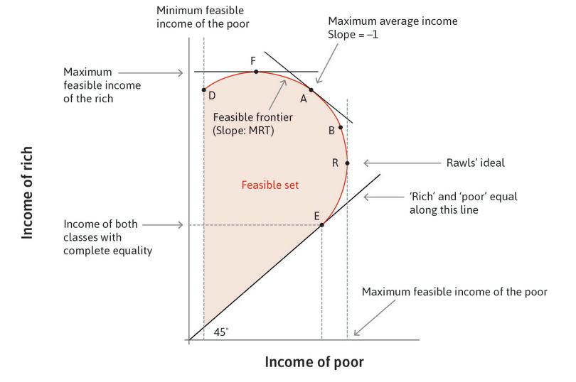
Like the feasible set when Angela and Bruno were bargaining in Unit 5, there is a minimum level of income that the poor can get. This minimum could be set by their biological survival needs, or perhaps by the fact that if income fell below this level they would revolt. Notice that if the poor were to be even poorer than at point F, the rich would also suffer. So like point E (maximal equality), point D (minimal income of the poor) is not Pareto efficient.
In the figure we have considered the following income distributions:
- E: complete equality
- R: the distribution with the highest income for the poor
- A: the highest average income of rich and poor
- F: the maximum income of the rich
- D: the distribution in which the poor are at their minimum feasible living standard
A preference for fairness
Which would you choose? Points between D and F are easy to eliminate from the running, as they are all inferior to point F for both classes. And the same goes for points between E and R. Eliminating all Pareto-inefficient distributions from consideration means that no points in the interior (inside) of the feasible set would be considered.
That leaves points between F and R. How will you choose among them? To answer this, you need to consult your indifference curves. In this case, an indifference curve gives combinations of the incomes of the two classes that you value equally.
Curves further away from the origin are preferred (more income for both groups is always better). The slope of these indifference curves is the marginal rate of substitution between income for the rich and income for the poor.
You would then maximize your utility by finding the point on the feasible frontier at which the marginal rate of transformation is equal to the marginal rate of substitution. If you wished to maximize your own expected income, then you would place an equal value on the income of the rich and the poor because you are equally likely to be one or the other.
- inequality aversion
- A dislike of outcomes in which some individuals receive more than others.
But you might care about the condition of the poorer class even if you were lucky enough to be assigned to the richer class in the coin flip (remember, you have to make your choice before you know your assignment). That is, you might be inequality averse, caring about your own payoffs but also disliking inequality across groups. In this case, you would have an indifference curve like the blue one shown in the figure. You would choose point B, somewhere between Rawls’ ideal (the highest feasible income of the poor) and point A, the highest average income.
The familiar graph of the feasible set and a family of indifference curves helps to clarify the choices about inequality and fairness that a citizen or group of citizens may wish to make. But it does not tell us how any of the points on the feasible frontier might actually be implemented. Changing the level of inequality in a society requires altering one or more of the causes of the current state of inequality. To understand income inequality, we first have to understand the factors that determine an individual’s income.
Question 19.5 Choose the correct answer(s)
Figure 19.15 shows the feasible frontier of the incomes of the rich and the poor.
Which of the following statements is correct?
- Point E is not Pareto efficient as at point R, both the rich and the poor are better off than at E. This reflects the belief that complete equality in society would remove incentives for its citizens to work, study, and take risks, so a little inequality could actually be better for all.
- The marginal rate of transformation, when negative, measures how much more income the rich receives per unit of income given up by the poor. This is the steepest at R.
- If you had a 50-50 chance of being rich or poor, then the average income is maximized at the point where the MRT = –1, that is, one unit loss of income for rich / poor leads to exactly the same gain for poor / rich (otherwise you would be able to increase the total income by choosing another point). This is point A.
- Between D and F, incomes of both the rich and poor decrease. This could occur because the rich have to dedicate resources to protecting their wealth from the poor, resulting in lower total output.
19.5 Endowments, technology, and institutions
Income and endowments
In this section, we provide a framework that helps explain why different individuals receive different incomes.
- endowment
- The facts about an individual that may affect his or her income, such as the physical wealth a person has, either land, housing, or a portfolio of shares (stocks). Also includes level and quality of schooling, special training, the computer languages in which the individual can work, work experience in internships, citizenship, whether the individual has a visa (or green card) allowing employment in a particular labour market, the nationality and gender of the individual, and even the person’s race or social class background. See also: human capital.
An individual’s income depends on things that they own, or are, or have that allow them to receive income. These things affecting a person’s income are called endowments and include:
- human capital
- The stock of knowledge, skills, behavioural attributes, and personal characteristics that determine the labour productivity or labour earnings of an individual. Investment in this through education, training, and socialization can increase the stock, and such investment is one of the sources of economic growth. Part of an individual’s endowments. See also: endowment.
- Their financial wealth: Their savings or stocks or bonds that they own, on which they receive interest or dividends.
- The physical assets they own: For example, land or the buildings and machinery of a company on which they may receive profits or rents, and which they can use as collateral.
- Their schooling and work experience, which affects their value to an employer and therefore their earnings on the labour market (sometimes termed their human capital).
- Their race, gender, age, and other aspects that may affect wages, access to credit, or other exchanges.
- Their citizenship and whether the individual has a visa, which determine whether they can legally work in a particular country and therefore their earnings on the labour market.
- Any other attribute, or possession, or capacity that affects the income an individual will receive.
As a result, we can think of an individual’s income as depending on:
- their endowments
- the income resulting from each item in the set of their endowments
So, for example, consider a person, Ella, whose endowment is the ability to work full time (1,750 hours) at a wage based on her skill as a medical technician (€30 per hour). She also receives a child benefit of €2,000 as an entitlement from the government for her child. Her endowment would be the following list:
- ability to work 1,750 hours of labour per annum as a medical technician
- the right to a child benefit to assist in caring for her child
She has been able to secure only half-time work (875 hours) so the annual income she derived from all sources is: (875 hours × €30) + (1 child grant × €2,000) = €26,250.
Now consider Kamal, who recently inherited a sum from his late father sufficient to start a small business. He was previously working as the manager of a similar small firm for €120,000 per year. Kamal’s endowment is:
- ability to work full time using skills and experience as a manager
- ownership of the buildings, equipment, and other assets of his firm, worth €8 million
If he did not manage the firm himself, he would have to hire a full time manager with similar skills and experience, costing him €120,000. Last year, his firm’s (accounting) profit was €600,000 without counting Kamal’s own efforts as a manager, worth €120,000 a year. So his income is the €600,000 in profit, which we divide into the returns to his managerial efforts (€120,000) and the returns to the ownership of assets (€480,000).
By studying why people have differing endowments, and what determines the income associated with each of the endowments, we can understand income inequality.
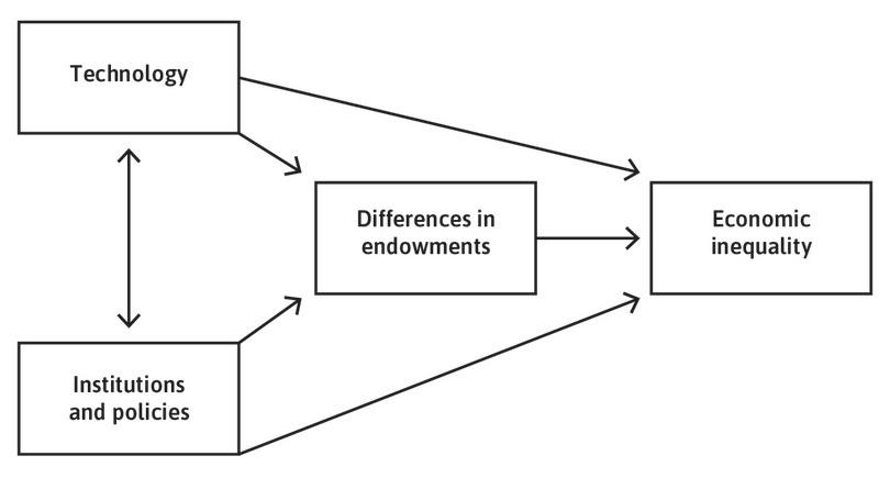
The factors influencing individual income can be understood using the model of cause-and-effect relationships in Figure 19.16. The arrows point from a cause to an effect.
Both institutions and technologies are part of the explanation of differing endowments among individuals. Inherited wealth gave Kamal a valuable asset, while subsidized higher education helped Ella qualify as a medical technician. Both are examples of the effect of institutions on endowments.
We have seen that intergenerational inequality will be greater where inheritances are not heavily taxed and where educational policies allow the wealthy to acquire more and better education for their children. If marriage customs result in spouses having similar levels of wealth—called ‘positive assortment’—this will contribute to inequalities in endowments. Elite private universities, for example, contribute to positive assortment because like exclusive social clubs, they provide meeting and matching opportunities for the sons and daughters of the wealthy. These are also examples of institutions influencing differences in endowments.
Technology matters, too. Where there are strong economies of scale such as in the technology of digital platforms, these will support the winner-take-all forms of competition that we explain in Unit 21. In this setting, a few people—the winners—will end up with substantial endowments in the form of valuable financial or real assets, while the rest end up with little.
The value of a particular endowment, say a programming skill or ownership of a 3D printer, depends on both technology and institutions, as well as on other factors, including supply and demand. The demand for Ella’s skill was limited, perhaps due to cuts in health care spending, so she was unable to work full time. Next year Kamal’s firm may face competition from a new competitor, making the 7.5% rate of return ($600,000/$8,000,000) that he made this year impossible. Both are examples of how institutions affect the income provided by an asset.
Technology matters, too. Being physically strong was a valuable endowment in agriculture—at least until mechanization made it less important in determining earnings. In that case a change in technology (mechanization) reduced the demand for a particular kind of skill, and so its value (relative to other skills) fell. The value of land, for example, will depend on how productive it is in growing marketable crops (technology) and whether it is zoned for commercial or residential uses (institutions).
Using the model to review inequality from previous units
In previous units, we studied how differences in endowments determined economic outcomes, including inequality. Figure 19.17 summarizes these situations, starting with the interaction in Unit 5 between Bruno, the landlord, and Angela, the farmer he employed.
Recall that how much Bruno got and the inequality between them depended on:
- Their endowments: The fact that Bruno owned the land meant he could exclude Angela from working on it
- Angela’s productivity as a worker: This is determined by Angela’s endowment of skills and capacities, as well as the available technology.
- Angela’s reservation option: What Angela would get if she were to refuse to work for Bruno or he refused to hire her. This is an important influence on her bargaining power in her dealings with Bruno. It is determined by her endowments and the institutions or policies in place.
The endowments of the pairs of individuals in Figure 19.17 appear in the second column of the figure. In the first example, Bruno owns the land and Angela only owns her time and capacity to work. This inequality in land ownership matters because it determines who has to work for whom, and who can earn income from allowing others to work with their capital goods or their land.
Endowments matter in another way, because they change Angela’s reservation option. If Angela owned land that she could work herself, then Bruno would need to pay her at least enough to ensure that she would rather work for him than work on her own land.
Recall that a change in institutions and policies can change Angela’s reservation option. Before the rule of law, the institutions were such that Bruno could simply coerce her to work, and the only thing that constrained the size of the surplus he could get was the need to keep Angela healthy enough to work the next day.
The institutional change, which gave her the right to say no, improved this reservation option. Bruno had to offer Angela a deal that would make her better off working for him than not working. Angela’s new ‘right to say no’ raised the value of her labour endowment.
| Situation, actors and unit | Endowment | Reservation option | Conflict over? | Institutions and policies (examples) | Technology (examples) |
|---|---|---|---|---|---|
| Landlord and farmer: Bruno and Angela (Unit 5) | Bruno owns the land; Angela has 24 hours of potential labour | Bruno: rent land to another farmer; Angela: government support | Rent paid by Angela to Bruno and the hours that Angela works | Angela’s reservation option (which depends on whether slavery is legal) and legislation limiting work hours. | Angela’s increased productivity due to an improvement in seeds allows Bruno a larger surplus when he has all the bargaining power. |
| Borrowing, lending and investment: Julia and Marco (Unit 10) | Julia: $100 next year; Marco: $100 now | Julia: consume nothing now, $100 later; Marco: consume some now, store and consume some later | Julia benefits from a low interest rate and Marco benefits from a high interest rate. | Competition among lenders and interest rate regulation | An improvement in storage technology (for example less loss of grain to the mice) makes it easier for Marco to move his goods forward in time, and also raises the rate of return on his investments. |
| Specialization and trade: Greta and Carlos (Unit 18) | The skills and resources of each that determine their feasible consumption set in the absence of specialization and trade | Both: the utility they would enjoy if they did the best possible without trading | Price at which they exchange the good in which they specialize when they trade | Price-setting power by either Greta or Carlos | An improvement in the technology of the good in which one specializes will benefit both, the larger gains going to the person with price-setting power. |
| Firm: owners and employees (Unit 6) | Owner: ownership of the firm; Employee: capacity to work given her skills | Owner: hire some other employee; Employee: unemployment insurance and job search | Wage, working conditions, effort on the job | Level of unemployment insurance, employment level, and legislation regulating work conditions | A new technology may increase the productivity of the employee’s effort, increasing the employer’s profits (short run) and increasing employment and the real wage (long run). It may also affect how easily the employer can monitor the employee’s effort. |
| Banana plantation: owners and downstream fishing communities (Unit 12) | Owners: the land and other capital goods of the plantation; Fishing communities: their boats and capacity to catch fish, access to fisheries | Owners: raise bananas without using Weevokil pesticide; Fishing communities: convert to farming | Use of polluting chemical, possible compensation for destruction of fisheries or commitment not to use Weevokil | Regulations governing the use of pollutants and enforcement of private agreements made between the parties | A new pesticide technology could reduce or increase the conflict between the two groups depending on its external effects. |
Inequality: Endowments, reservation options, conflicts, institutions, and technologies.
Figure 19.17 Inequality: Endowments, reservation options, conflicts, institutions, and technologies.
In the last column of Figure 19.17 we consider the way that changes in technology affect the degree of inequality. In the row concerning the firm’s owners and employees, a labour-saving technology, as we saw in Unit 16, can—at least initially—reduce the number of workers a firm needs, making employees more vulnerable to job loss and reducing the likelihood of getting another job at the same wage for those who have been fired.
Like technology, institutions and policies affect the value of endowments. In the example of Ella, the medical technician, her specialized skills are part of her endowment but their paid value (€30 per hour in the example) will depend on institutions. If gender discrimination is a common practice of employers, then her skills might be worth less. If a license is required to do this work, then the value of her skills will be greater if she is licensed. These are examples of institutions and policies affecting the value of endowments.
The credit market in Unit 10 is another example. Recall that Julia’s endowment is $100 next year. What she can consume now depends on her wealth (what is in the bathtub), and that depends on the institutions and policies determining whether she can borrow, and the interest rate at which she can borrow.
If her only option is the village moneylender in Chambar or a payday lender in New York, she faces a high interest rate and her wealth (now) is much lower than $100. If she can borrow at a low interest rate, her wealth is quite close to $100. If she can’t borrow at all, then there is nothing in the bathtub and her wealth now is zero.
How endowments, technology, institutions, and inequality interact over time
Endowments and the income that they provide are constantly changing as people acquire more skills or as the value of some endowment—such as a piece of land or a rental apartment—falls. Figure 19.16 illustrated the causes of economic inequality. In Figure 19.18, we illustrate inequality as a cause of changes in institutions, technology, and differences in endowments.
The arrow from economic inequality to differences in endowments in the next period captures the fact that the children of richer parents may end up with more and higher quality education, or with greater inherited wealth.
Economic inequality over time. The red arrows show that economic inequality in one period has effects on technologies, institutions and policies, and differences in endowments in the future.
Figure 19.18 Economic inequality over time. The red arrows show that economic inequality in one period has effects on technologies, institutions and policies, and differences in endowments in the future.
Economic inequality may also influence institutions and policies. An example we shall see in Unit 22 is that in most countries—even democracies—a wealthy person typically has more influence on what the government does than does a poor person. A greater gap between the rich and the poor could increase the political advantage of the wealthy, resulting in policies favouring those with higher incomes.
Exercise 19.7 Yichen, Renfu, Mark, and Stephanie
Consider the economic situation of Yichen, Renfu, Mark, and Stephanie, discussed at the start of this unit. Give examples of how technology, institutions, and differences in endowments explain economic inequality between these actors, and how inequality between them could change over time.
19.6 Inequality, endowments, and principal-agent relationships
Recall that the labour and credit market models in Units 9 and 10 provided the background for our macroeconomic models of the functioning of the whole economy and for the study of how shocks and policies affect economy-wide employment, incomes, and inflation. We used the Lorenz curve to summarize the effects on inequality. And in explaining the model of inequality in Figure 19.16, we used examples from the labour and credit markets.
- principal-agent relationship
- This relationship exists when one party (the principal) would like another party (the agent) to act in some way, or have some attribute that is in the interest of the principal, and that cannot be enforced or guaranteed in a binding contract. See also: incomplete contract. Also known as: principal-agent problem.
The principal-agent models also give us a new way to study an important dimension of inequality: differences in power affect the type of choices that a person may feasibly make. Principals are in a position to exercise power over agents, but agents rarely can exercise power over principals. Here is why.
The employer (the owner or the manager who is the principal in the labour market) has the power to determine what the firm will produce, using what technology, and in which country to locate production. They also have the power to set the wage and the tasks that a worker is directed to perform, and can also fire the worker. The worker chooses how to go about her work within limits that the employer sets.
Recall that in order to motivate the worker to work hard and well, the employer sets a wage so that the employee is better off with the job than she would be without it, receiving an economic rent. The employer can fire the worker and deprive her of the employment rent she would otherwise receive. The fear of losing this rent is an important reason for the worker to carry out the employer’s wishes. It is also the reason why the employer has power over the employee.
The worker could, of course, quit. But this does not make the relationship equal when it comes to power. If she is receiving an economic rent she would penalize herself by quitting, and her employer would just replace her with someone currently unemployed.
We can contrast this with the relationships among price-taking buyers and sellers at the equilibrium of a competitive market. None of these traders is in a position to demand that any other trader act in one way or another. Think about the buyer, for example, who orders the seller to make the good available at a lower price, threatening not to buy otherwise. What would the seller do? Nothing. The seller can sell as much as she wishes at the going price (remember, the demand curve facing an individual firm is flat).
A second contrast is with the interactions we studied in Unit 4 where the actions open to all parties were identical—for example, either use integrated pest management or chemical fertilizers, either learn C++ or Java.
Like the relationship between the employer and employee, the other principal-agent models we have seen reflect the unequal relationships between groups of people with differing endowments, such as landlords and tenant farmers, and borrowers and lenders.
Figure 19.19 illustrates how the credit and labour markets influence the relationships among the groups of lenders and borrowers, and employers and employees.
Starting at the upper left of the figure, wealthy individuals can use their wealth to purchase the capital goods to become employers and they can also lend to others. Among the less wealthy, there will be some successful borrowers who can as a result also become employers. Those with even less wealth cannot borrow (they are the credit market excluded that you studied in Unit 10, or can only borrow where the house provides the collateral for the mortgage), and must seek work as employees. Employers then hire employees from among the less wealthy, with some remaining unemployed (due to the workings of the labour market that you studied in Units 6, 9, and 15).
Horizontal arrows indicate a principal-agent relationship. Lenders and employers are the principals in the figure; their common red colour indicates this similarity. Agents—successful borrowers, and employees—are coloured green to distinguish them from would-be agents (credit market excluded and unemployed) who are coloured purple. You definitely do not want to be in the purple boxes. But even if you are an agent lucky enough to be in one of the green boxes, the principal can put you back in the purple box just by refusing to deal with you. This is why lenders and employers have power over borrowers and employees.
Figure 19.19 helps us understand why some people end up as principals (employers, for example) while others end up as agents (employees). If one is wealthy, one can be both a lender and an employer. There is some truth to the saying that ‘people are born into their position in the economic order’. This was literally true in some economies of the past. For example, the position of the slave was perpetuated by the enslavement of their children as a matter of law.
Something similar can occur in places where wealth is inherited from parent to child. The children of employees (who inherit little wealth) are also more likely to become the next generation’s workers than are the children of employers. You already saw that the children of well off parents in the US also tend to have high incomes when they become adults (Figure 19.10).
But look again at that figure: there is some mobility among the income groups even in the US and there is very little intergenerational inequality in Denmark. Becoming an employer requires that one has sufficient wealth. But inheriting wealth from a parent is not the only way, and in some countries not even the most important way to acquire wealth. The wealth necessary to become an employer may be acquired by saving. It may also be acquired by developing a great project and persuading investors called ‘venture capitalists’ to fund it.
We have also seen in Units 13 and 16 that there are transitions by individuals between boxes over their life-time. A younger person may initially be a borrower and then be a lender later in life; a spell of unemployment can be followed by one of employment.
Question 19.6 Choose the correct answer(s)
Which of the following statements are correct?
- This is the definition of endowment.
- Whether one has a degree or not affects the income of the individuals. Therefore one with a degree and one without have different endowments.
- Reservation options depend on the individuals’ endowments. For example, a firm owner’s reservation option is to hire another employee, while an employee’s reservation option is receiving an unemployment benefit.
- Marketability is not part of the definition of an endowment. An endowment is anything—including the right visa—that can affect an individual’s income.
19.7 Putting the model to work: Explaining changes in inequality
The model presented in the previous section helps us to understand why individuals have different incomes. To understand inequality, however, we need to consider the changes across the entire income distribution. In this section, we will apply the labour market model from Unit 9, in combination with our understanding of the determinants of individuals’ income, to look at the effect on inequality of:
- an increase in the educational level of the workforce
- a reduction in discrimination against a segment of the workforce
- automation of production reducing the demand for some skills and increasing others
You may wish to review the workings of the labour market model described in Unit 9 before proceeding.
A more educated and more productive workforce
What will be the consequences if workers have acquired more schooling? We expect additional schooling to increase productivity, meaning that a unit of effort by a more educated worker produces more goods per hour using the same technology. The direct effect of additional schooling on an individual is therefore to improve their endowment of labour. Holding everything else equal, the increased productivity means that any individual can get paid a higher wage for their labour.
However, what if the entire workforce becomes more educated? This could be the result, for instance, of an increase in the compulsory schooling age. At the pre-existing real wage, the result of higher productivity will be a higher profit for the firms. This shifts the price-setting curve upwards, as shown in the left panel of Figure 19.20. With higher profits, new firms enter and existing firms hire additional workers, which reduces the unemployment rate. Lower unemployment in turn makes it easier for a dismissed worker to find a new job. It therefore increases the workers’ reservation position, raising the wage. Workers both possess a better, higher-productivity endowment of labour time and enjoy better prices for their endowment.
The effects on inequality are shown in the right panel of Figure 19.20. There are now fewer unemployed workers. The segment of the Lorenz curve representing employed workers is now flatter because even though the real wage has risen, a larger fraction of the work force (85% instead of 80%) receives the same 60% of the (now increased) total output.
The line segment for the owners is unaffected because the same 10% of the population continue to receive 40% of the output; like the wages of workers, their profits are up because more is being produced. In this example, the effect of the increased education and productivity of the workforce on inequality is to reduce the Gini coefficient from 0.36 to 0.33.
A reduction in labour market segmentation
- primary labour market
- A market in which workers are typically represented by trade unions, and enjoy high wages and job security. See also: secondary labour market, segmented labour market.
Until now we have assumed that all workers receive the same wage in a single labour market, but in reality there are many distinct labour markets. In what is termed the primary labour market, workers may be represented by trade unions, and enjoy high wages and job security. ‘Job ladders’ allow promotion to better paying and more secure jobs. Primary labour market jobs are frequently referred to as ‘good jobs’.
- secondary labour market
- Workers typically on short-term contracts with limited wages and job security. This might be due to their age, or because they are discriminated against by race or ethnic group. See also: primary labour market, segmented labour market.
Workers in the secondary labour market are on short-term contracts with limited wages and job security, and tend to be young or from populations discriminated against by race or ethnic group. In many European countries, these are called ‘zero-hours contracts’ because the employer does not commit to providing work for any particular number of hours. The secondary labour market is also referred to as the ‘gig economy’ in which freelance work or very short-term contracts are the norm, rather than permanent jobs. For any given endowment of skills, these workers will usually receive a lower income than the workers in the primary labour market. Institutions therefore benefit the workers in the primary labour market and disadvantage workers in the secondary market, increasing income inequality.
- segmented labour market
- A labour market whose distinct segments function as separate labour markets with limited mobility of workers from one segment to the other (including for reasons of racial, language, or other forms of discrimination). See also: primary labour market, secondary labour market.
Figure 19.21 shows a Lorenz curve for an economy with labour market segmentation, with a low-wage segment and an equal number of high-wage primary segment workers. The owners are not segmented because they can easily invest their wealth in firms in either or both sectors and, as a consequence, the rate of return will be the same in both sectors. The elimination of labour market segmentation means that all workers receive the same wage, but unless this affects the relative bargaining power of workers and owners, it does not alter the share of the output going to workers as a whole. This demonstrates how institutional change can reduce inequality by aligning the wages individuals receive for their endowments.
The figure illustrates the fact that much of the inequality in modern economies is among employees (from secondary labour market workers to very highly paid professionals), and that reducing these inequalities can significantly reduce the Gini coefficient. Where trade unions have reduced labour market segmentation and narrowed the wage differentials among workers, inequality is lower. An example is the so-called solidarity wage policy introduced in Sweden, which we will discuss in Unit 22.
Automation
- automation
- The use of machines that are substitutes for labour.
Automation is a term used to describe new technologies that allow machines to do the work that people used to do. Technological innovations that replace labour have been an essential part of the capitalist economy since the introduction of the spinning jenny in the eighteenth century, which we described in Unit 2. As we saw in Unit 16, new technologies typically put some people out of work, while increasing the demand for the skills of other workers. We can study these effects using the Lorenz curve and the Gini coefficient derived from it.
To see how, consider a hypothetical economy in Figure 19.22, before and after it introduces machines that perform routine operations that had always been done by humans. We’ll call these machines ‘robots’. The solid blue Lorenz curve depicts the distribution of income between five employers and 95 workers before the introduction of the robots. Five of the workers are unemployed, and among the 90 who are employed, all receive the same wage, whether they do routine or non-routine work.
The slope of the flatter of the two upward-sloping lines is an indication of how much workers are paid relative to their productivity. We see that the 90 employed workers receive 60% of the income of the economy. So each receives 0.60/90 or two-thirds of a per cent of what the economy produces. The slope of the steeper solid line shows that five owners receive 40% of the income, so that each receives 8% (= 0.40/5) of the output of the entire economy.
To understand the short-run impact of the plan to introduce robots, think about the skill endowments of the workers. Sixty of them are doing routine jobs that were once relatively well paid, such as machine tending or mail sorting, that can now be done by robots. Others have the training to not just operate machinery, but to design, repair, and calibrate machinery, and manage its deployment.
The short-run effects depend on the kinds of work a worker does:
- The robots are labour-replacing: For routine jobs in which the machines and skills are substitutes, the value of a worker’s endowment is reduced by the new technology because the robot can replace the worker.
- The robots are labour-enhancing: For those jobs in which the machines and skills are complements, the value of a worker’s endowment is increased by the new technology.
These two effects are shown in the new (dashed) Lorenz curve depicting the short-run effects of the new technology on workers who previously earned two-thirds of a per cent of output each. At least some of the 60 workers for whom the robots are labour-replacing lose their job. Five of them have now joined the unemployed; the machines have replaced their labour. Those who remain employed have suffered a fall in their bargaining power (because they too can be replaced). These 55 workers now receive 25% of the output of the economy, and their earnings fall to 0.5% of the total output each.
On the other hand, the 30 workers with skills that are complementary to the robots have gained. They now receive 35% of the output of the economy, or a little more than 1% each.
The effect of automation thus can be similar to the effect of labour market segmentation, but in the case of robots, the segregation of workers depends on whether their skills are easily substituted by machines (the losers) or instead are complementary to the machines (the gainers).
The result is that the Gini coefficient increases from 0.38 to 0.53, shown by the new Lorenz curve falling further below the perfect equality line.
An example of the effect of automation is the introduction of automatic teller machines (ATMs) by banks. Surely this would have increased unemployment among human bank tellers?
James Bessen, an economist, looked at the employment levels in the US and found that the number of bank tellers continued to rise even after the machines were installed. Rather than doing mechanical tasks, they were now providing other services such as advice to customers.10
Bessen also found employment increased among bookkeepers and retail sales staff despite automation of some of their tasks, but on the other hand, technology did displace the jobs of travel agents. Automation was complementary to the skills of some bookkeepers and bank tellers, but it was a substitute for the skills of travel agents.
Listen to James Bessen talk about his book in a May 2016 episode of the EconTalk podcast.
What determines whether automation increases or decreases wages and employment? We can use an analysis similar to the one we did in Unit 16. There are two contradictory effects.
On one hand:
- Labour-replacing automation reduces the demand for some types of labour: this sends workers into unemployment.
- This reduces the reservation option of all workers: It lowers the wage that firms have to set to maintain their desired level of work effort.
On the other hand:
- The increase in labour productivity increases profits.
- This motivates and finances an expansion of the capital stock of the economy.
- The increase in capital stock creates additional employment opportunities: It reduces unemployment and increases the wage required to motivate workers along the wage-setting curve.
As we saw in Unit 16, adjustment of local labour markets to labour-saving technology and competition from imports may take a very long time.
The model cannot determine whether the new Nash equilibrium in the labour market will result in a more equal distribution of income or a less equal one. Inequality among workers will be greater due to the fact that the robots created winners and losers among employees, by raising the value of some labour endowments (the engineers) and lowering the value of the labour endowments of others (the routine workers). If the level of unemployment goes back down to its pre-automation level, and if the firm’s markup on costs is unaffected, then the only durable effect will be greater inequality among workers, resulting in an increase in the Gini coefficient.
A government observing the process of automation might respond with levying taxes on the enhanced profits of the owners and on the incomes of the workers with increased wages. In designing the taxes, it would need to take into account their effect on the behaviour of workers and employers. The revenue from these taxes can be used to finance:
- Additional employment and opportunities for career progression and rising wages: These opportunities could be in human services such as health and care, where jobs are non-routine but often poorly paid.
- Opportunities for workers with routine skills to upgrade their endowments: Their labour becomes machine-enhanced rather than machine-replaceable; for example, a former drill press operator learning how to code.
Exercise 19.8 How automation affects employment
Return to Figures 19.6 and 19.7. Use what you have learned in this section about robots as substitutes or complements to employees’ endowments to explain some of the patterns in job growth shown in these figures.
Question 19.7 Choose the correct answer(s)
Which of the following statements regarding segmented labour markets are correct?
- The ‘gig economy’ is part of the secondary labour market.
- Workers in the primary labour market enjoy higher wages and job security, while those in the secondary labour market have lower wages and limited job security.
- When trade unions negotiate with employers over working hours, employers have to guarantee that employees can work for the agreed number of hours. This is different from zero hours contracts, in which the employer does not commit to providing work for any particular number of hours. Zero hours contracts occur in the secondary labour market, which is not protected by trade unions.
- Primary labour market jobs are those that are well-represented by trade unions, and have high wages and job security. Thus, while some agricultural jobs fall into this category, a greater proportion of primary labour market jobs are professional (white-collar) jobs.
19.8 Predistribution
- redistribution policy
- Taxes, monetary, and in-kind transfers of the government that result in a distribution of final income that differs from the distribution of market income. See also: predistribution policy.
- predistribution policy
- Government actions that affect the endowments people have and their value, including the distribution of market income and the distribution of privately held wealth. Examples include education, minimum wage, and anti-discrimination policies. See also: redistribution policy.
- statutory minimum wage
- A minimum level of pay laid down by law, for workers in general or of some specified type. The intention of a minimum wage is to guarantee living standards for the low-paid. Many countries, including the UK and the US, enforce this with legislation. Also known as: minimum wage.
Governments influence the degree of inequality in the economy. They do this in two ways:
- Redistribution: By taxes and transfers that result in a distribution of disposable income that differs from the distribution of market income (as we saw in Figure 19.1) and by expenditure that provides public services to households.
- Predistribution: By affecting the endowments that people have and the value of those endowments, leading to a change in the inequality in market income (going back to Figure 19.1 again, here governments affect the distribution of earnings before taxes and transfers or the distribution of privately held wealth).
Examples of predistribution that you have already seen include:
- Increased education of the workforce: This changes the endowments of employees, adding skills and other work relevant capacities that will affect market incomes.
- Eliminating or reducing labour market segmentation: This—and other anti-discrimination policies—will alter the prices (wages) that a person’s endowment will be paid in the labour market. In particular, it raises the value of the endowments of people who otherwise would suffer discrimination.
Other aspects of predistribution affect the basic institutional structure of the economy. By defining and enforcing the legal framework in which the employers, banks, employees, unions, borrowers, and other key economic actors interact, governments affect the distribution of market income. Using the legal system, governments can also alter which property rights are protected, for example banning slavery, legalizing unions (Units 9 and 16), establishing trading rights in emissions (Unit 18), or setting the duration of intellectual property rights and patents (Unit 21). All of these measures can change the relative bargaining power between groups as well as their reservation options, which in turn will change the distribution of income.
Finally, governments can change the set of contracts that are allowed, which alters the distribution of income. We discussed one example in Unit 5, when we saw the effect of legislation that limited the maximum hours that employees could work.
Another important example of predistribution by limiting the kinds of contracts that are allowed is a statutory minimum wage, which prohibits contracts with wages below a certain level. This affects the value of a worker’s endowment of labour, but it may also affect the likelihood that the worker will be able to find a job. The costs of the minimum wage could be fewer jobs.
Arin Dube, an economist, studied differential changes in minimum wages in bordering local areas in the US.11 In our ‘Economist in action’ video he explains that he found that raising the minimum wage had a little negative impact on employment but increased the income of poor workers on average.
Ensuring high-quality early childhood education is another predistribution policy.12 In our ‘Economist in action’ video, James Heckman, a Nobel-prize-winning economist from the University of Chicago, shows how economists can learn from experiments and other data about how to level the playing field for children growing up poor.
Figure 19.23 lists a set of policies that can reduce inequality in market incomes, drawn from this and other units.
| Endowment | Policy | Direct effect | Indirect effect | Unit |
|---|---|---|---|---|
| Labour | Free high-quality primary education for all children | Increases opportunities for poorer children to attain more advanced levels of schooling, which increases the market value of their endowment of labour | Raises average productivity of labour, shifting up price-setting curve, which increases wages and employment (ceteris paribus) | U19 |
| Labour | Raise the share of the harvest going to the farmer | Increases the value of the farmer’s endowment of labour | Raises farmers’ incomes | U5 |
| Labour | Eliminate ethnic, racial, or gender discrimination | Increases the value of the labour endowment of those targeted by discrimination | Raises incomes of targeted groups | U19 |
| Labour | Minimum wage | Increases value of labour endowments among those who were previously unable to work for more than the minimum wage | Raises incomes of the poor and reduces incomes of employers (unless employment effects dominate) | U19 |
| Labour | Laws and policies to increase workers’ bargaining power (for example trade unions) | Increases value of labour endowments of trade union members and improves working conditions | Raises incomes of trade union members (unless negative employment or productivity effects dominate) and reduces incomes of employers | U9, U16, U19 |
| Ownership of firms | Policies to ensure competition | Reduces price markup | Raises real wages, reduces profits | U7, U9, U16 |
| Intellectual property | Restrict IPRs (for example shorter patents or copyrights) | Reduces value of endowment of intellectual property among IPR holders. | May discourage innovation but enables quicker diffusion of innovations | U21 |
| Professional license | Allow easier access to licenses (for example for taxis) | Increases supply and reduces incomes of license holders. | Greater equality (if license holders are richer than average) | U19 |
Predistribution policies that can reduce inequality in market incomes.
Figure 19.23 Predistribution policies that can reduce inequality in market incomes.
- non-compete contract
- A contract of employment containing a provision or agreement by which the worker cannot leave to work for a competitor. This may reduce the reservation option of the worker, lowering the wage that the employer needs to pay.
Exercise 19.9 Non-compete contracts in the labour market model
Legislation can rule out particular kinds of contracts, such as those that prohibit employees from leaving their firm to work for a competitor. The justification offered for these non-compete contracts is that workers leaving a firm may take with them industrial or trade secrets that would benefit the competition. But in the US, non-compete clauses are even included in contracts of fast-food workers. Use the labour market model to explain why employers would introduce non-compete contracts in sectors where industrial secrets are not an issue.
Question 19.8 Choose the correct answer(s)
According to our ‘Economist in action’ video of Arin Dube, which of the following was a finding of his study of the minimum wage increase?
- This could be true, but is not stated in the video.
- This could be true, but is not stated in the video.
- This could be true, but is not stated in the video.
- This is definitely stated in the video.
Question 19.9 Choose the correct answer(s)
Watch our ‘Economist in action’ video of James Heckman. According to Heckman, which of the following individual attributes are NOT among the reasons for persistent poverty in a family from generation to generation?
- Inherited IQ could contribute to persistent poverty, but it is not mentioned in the video.
- Heckman argues that this is among the reasons for persistent poverty.
- Heckman argues that this is among the reasons for persistent poverty.
- Heckman argues that this is among the reasons for persistent poverty.
19.9 Explaining recent trends in inequality in market income
Can these policies or other changes help explain the trends in market income inequality? Figure 19.24 indicates three of these trends and suggests possible explanations based on the models you have learned.
| Trends | Data | Contributing causes | Models |
|---|---|---|---|
| Declining within-country inequality (1920–1980) | Figures 19.2, 19.3, 19.4 | Increasing education and productivity reduced unemployment. Reduced labour market segmentation and other sources of inequality among workers. Technological improvements that were complementary to low and middle-skill workers. |
Figure 19.20, Figure 19.21 |
| Stable or rising within-country inequality (1980–2017) | Figures 19.2, 19.3, 19.4, 19.6, 17.3 (upper panel) | Increased inequality among workers due to new technologies that were complementary to the skills of higher paid workers, and substitutes for workers doing routine tasks. Weaker trade unions and conservative political parties in power saw bargaining power shift in favour of employers, whilst the resulting higher profits after taxes were not translated into expanding employment (in some countries). |
Figure 19.22 |
| Stable or decreasing between-country inequality (1995–2017) | Figure 19.5 | Reduced global labour market segmentation due to rapid growth of labour productivity and demand in China and other poorer countries. | Figure 19.24 |
Using economic models to explain trends in inequality in market income.
Figure 19.24 Using economic models to explain trends in inequality in market income.
To explain the reduction in between-country inequality (and the associated reduction in between-household inequality) in the world, think of the world as a single capitalist economy with a labour market that is segmented along national lines. To do this, we propose a very simple economy of the ‘world’ with just two ‘countries’: China and Europe-and-North-America. So instead of two labour market segments in the same country, there are two countries, a low-wage country and a high-wage country, a little like China and the US in Unit 18.
Just as it is not easy for workers to move up from the secondary to the primary labour market within a country, the global economy has nationally segmented labour markets because of the barriers facing workers who would like to relocate from one country to the other. And, just as in the national economy, owners are not segmented. They invest their wealth wherever it will get the highest return. As we saw in Unit 18, globalization is only partial: the world labour market is far from integrated while capital mobility is high, because money does not need a green card or a work visa to be allowed to ‘work’ in a country.
The process of globalization has been associated with a reduction in global labour market inequality, as the once-low wages in successful exporter countries like China begin to catch up with wages in the higher-wage economies like France. A second effect has been a vast increase in the amount of labour that is now available for employment in the global capitalist economy, and this has been associated with an increase in the share of income going to owners of firms rather than employees.
19.10 Redistribution: Taxes and transfers
Differences among economies in the extent and nature of redistribution
Our models of wages and profits try to explain market income. But that is not the amount of income that people have to spend, nor does it include things essential to our livelihoods that we do not purchase, but instead acquire as a matter of citizenship.
Disposable income, as you know, is the income a person has after paying any income taxes and social security contributions, and after receiving any government transfers. But this is not an adequate measure of a household’s living standard because it does not include the effects of indirect taxes, such as value added tax, and the extent to which free or subsidized public services such as public education and health are available to households.
- in-kind transfers
- Public expenditure in the form of free or subsidized services for households rather than in the form of cash transfers.
These public expenditures are called in-kind transfers because they are a transfer to households in the form of free or subsidized services, rather than in the form of cash. When we take into account both indirect taxes and in-kind transfers, we arrive at a third income concept, called final income. Final income is the most complete measure of the living standard of a household. It tells us the value of all the goods and services that the household is able to consume. Figure 19.26 summarizes the relationship between these three income concepts.
Figure 19.27 shows the Gini coefficients for market income, disposable income, and final income for three large middle-income countries. In South Africa, direct taxes and transfers reduce the Gini by 0.08, from 0.77 to 0.69. Indirect taxes and public services reduce the Gini by a further 0.09 to 0.60 for final income, but it remains exceptionally unequal. Brazil had much higher inequality than Mexico in both market income and disposable income, but the Gini coefficient for final income falls to almost the same level as Mexico’s, at 0.44 compared to 0.43.
Gini coefficients for market income, disposable income, and final income.
Figure 19.27 Gini coefficients for market income, disposable income, and final income.
Nora Lustig, Carola Pessino and John Scott (2014), ‘The Impact of Taxes and Social Spending on Inequality and Poverty in Argentina, Bolivia, Brazil, Mexico, Peru, and Uruguay: Introduction to the Special Issue’. Public Finance Review Vol. 42 (3): pp. 287–303; Gabriela Inchauste, Nora Lustig, Mashekwa Maboshe, Catriona Purfield and Ingrid Woolard. (2015). ‘The Distributional Impact of Fiscal Policy in South Africa’. Commitment to Equity Working Paper No. 29, February 2015.
The welfare state
- welfare state
- A set of government policies designed to provide improvements in the welfare of citizens by assisting with income smoothing (for example, unemployment benefits and pensions).
The policies that turn market income into final income are often referred to as the welfare state. These policies can be broken down into the taxation side and the expenditure side. The taxation side is any policy that collects revenue for the government, while the expenditure side is any policy that either gives money to households, or spends money on their behalf. We will see more about the composition of government expenditures in Unit 22.
In countries where redistribution reduces inequality by a lot, most of this work is done by expenditures, rather than taxation.
In the 28 countries in the European Union, the average Gini in 2015 for market income is 0.46, which taxes and transfers reduce to 0.27 for disposable income. But taxes only achieve 0.04 of that redistribution, with the remaining 0.15 driven by transfers to households. This doesn’t mean that they have low tax rates, but instead it means that rich and poor pay similar shares of their incomes in taxes. On the other hand, poorer households benefit proportionally much more from expenditures.
Data on the Gini coefficient for the EU was taken from ‘Effects of tax-benefit components on inequality (Gini index), 2011–2015 policies’, which you can access on the Euromod statistics website.
Transfers, both in cash and in kind, have a large impact on inequality. But in most cases this is not their purpose. Most transfers are justified for other reasons, and reducing inequality is just a desirable side effect. Public education, for instance, has many justifications, including as an investment in human capital that makes the country more productive. Public health subsidies are often justified on the basis of a basic human right to life and to good health.
The welfare state is often represented and debated as a system of redistribution from the rich to the poor. But it is equally seen, and often defended, as redistribution from the lucky to the unlucky. Parts of the welfare state also redistribute from the young to the old.
- social insurance
- Expenditure by the government, financed by taxation, which provides protection against various economic risks (for example, loss of income due to sickness, or unemployment) and enables people to smooth incomes throughout their lifetime. See also: co-insurance.
In countries with large welfare states, much of the expenditure is on forms of social insurance, which includes assistance to poor households, but also includes public pensions, unemployment benefits, social housing, child benefits, and other expenditures that are targeted at groups that are not defined by low income. Public pensions transfer income to the old. Child benefits, like expenditures on public education, transfer income to the young (or those who care for them). Since they are paid for by taxes contributed by working adults, they are a way for society to enable people to smooth incomes throughout their lifetimes. We receive income from the government when we are very young and very old, when our incomes are low or zero, and we pay some of it back to the government when we are of working age and receiving a salary.
Similarly, public unemployment insurance is a way for people of working age to smooth their incomes in the face of the risk of unemployment. We pay while we are working, and we receive payments if we are out of work.
These forms of social insurance are not targeted specifically at poor people. But they have a large impact on inequality because most retired people and unemployed people would be very poor if they did not receive social insurance payments. In fact, in the European Union, public pensions are the policy with the greatest impact on inequality. They reduce the average Gini coefficient by 0.11, more than all other transfers combined.
Figure 19.28 shows the average household market income and disposable income in the UK in a single year, by age of the household’s primary earner. Households whose primary earner is less than 25 years old have an average household market income of £24,108 and an average household disposable income of £24,735. The richest group of households is those whose primary earner is aged 40–44 years old, and incomes decline rapidly after 60–64 years, as primary earners tend to retire. Disposable income is higher than market income for the under-25s and the over-65s, when market income is at its lowest, and conversely for those aged 25–64, when household income is at its highest.
If we hypothetically imagine that there is one household at each age group, the Gini coefficient for market income would be 0.249 while for disposable income it would be 0.139—the tax and benefit system as a whole reduces inequality because it effectively redistributes from richer households to poorer households. But the figure demonstrates that much of this result could be due to redistribution from those of working age to the retired.
Average household market and disposable income of households with primary earners in different age groups.
Figure 19.28 Average household market and disposable income of households with primary earners in different age groups.
Effects of taxes and benefits on household income. 2014/15. Office for National Statistics (UK).
How economists learn from facts What is the best way to give money to the poor? Randomize and find out.
Most countries adopt some policies to raise the living standards of the poor. But what is the best way to do this? If governments would like to transfer funds to individuals or families, should it go to the very poor, or only those who are working, or only those attempting to find work? Should the transfer be given to just the poor, or everyone?
The questions are controversial, and the answers will depend on more than economics. But economists have been using experiments to illuminate at least the costs and benefits of different mechanisms.
Economists have explored the effects of simply giving away cash to the poor, without requiring that they work or make any repayment. In theory, cash payments that one receives whether or not one is employed should have little impact on labour supply. Experiments have found that cash grants are a remarkably cost-effective way of reducing poverty on many dimensions, from increasing consumption to decreasing stress levels. These results have led policymakers to rethink their programs, for example, by comparing the anti-poverty effect of a dollar spent on, say, job training programs, with the effect of simply giving that dollar away.
Some have proposed to expand the cash payment to everyone, not just the poor, in what has been called Unconditional Basic Income Grants (UBI or BIG). Some Silicon Valley groups are funding initial experiments in these more universal cash grants in Oakland, California, randomizing access to cash. Some of them believe that technology is accelerating at such a rate, reducing labour demand to such an extent that universal income grants are going to be needed to keep the vast bulk of humanity from destitute unemployment.
Another proposal in Finland randomly selects betwen 2,000 and 3,000 people to receive monthly lump-sum payments of $600 to see if basic income grants can lower poverty as well as simplify the administration of programs to help the poor. Experimenting with a policy before adopting it wholesale is allowing economists to study some of the effects of particular policies, as well as letting policymakers use evidence to decide whether or not to adopt a policy.
Progressive and regressive redistribution
- progressive (policy)
- An expenditure or transfer that increases the incomes of poorer households by more than richer households, in percentage terms. See also: regressive (policy).
- regressive (policy)
- An expenditure or transfer that increases the incomes of richer households by more than poorer households, in percentage terms. See also: progressive (policy).
- distributionally neutral
- A policy that is neither progressive or regressive so that it does not alter the distribution of income. See also: progressive (policy), regressive (policy).
When the direct effect of a tax or transfer policy (compared to what would happen in the absence of the policy) is a reduction in inequality, it is called progressive. We have just seen that expenditures are more progressive than taxes. If a policy’s direct effect is a rise in inequality it is called regressive. Policies that are neither progressive nor regressive are called distributionally neutral.
For an expenditure or transfer to be progressive, it has to increase the incomes of poorer households by more than richer households, in percentage terms. This guarantees that it will reduce the Gini coefficient, and lead to a shift upwards in the Lorenz curve. Note that this policy might mean that in absolute terms (in units of currency), the richer households are receiving more.
Consider Bruno, the landlord, and Angela, the farmer. Suppose that the outcome of their bargaining is that Bruno’s income is three times as large as Angela’s, with Bruno receiving 3,000 pesos per year and Angela receiving 1,000. Suppose also that Angela has two children and Bruno three, all of whom go to publicly funded schools, and that the government spends 200 pesos per year per child. This means that Angela receives in-kind transfers worth 400 pesos per year and Bruno 600. For Angela this implies an increase in her final income of 40%. For Bruno, it is an increase of only 20%. So the transfer is progressive, and the Gini coefficient for final income will decline.
If it seems odd that the Gini will decline even if Bruno receives more than Angela, the explanation is that the Gini coefficient depends on relative incomes, or the ratios of incomes between households. Bruno’s market income is three times Angela’s market income. A policy that reduces that ratio will reduce the Gini coefficient. In the second case above, Bruno’s final income was 3,600 pesos while Angela’s was 1,400, which gives a ratio of 2.57 compared to 3 for market income. Even though Bruno received more in absolute terms, relative inequality between them declined, so the Gini coefficient declined.
Primary schooling is usually very progressive. A case of education expenditure that can be regressive is publicly funded university education. This is because children from richer families are much more likely to go to university. So if Bruno’s and Angela’s children were all of university age, but Bruno’s children were attending university while Angela’s were working, then public university spending would be regressive: Angela’s family would receive nothing, while Bruno’s would receive something.
When it comes to taxes, an analogous principle applies. A tax is progressive if richer households pay a larger share of their incomes than poorer households, and regressive if poorer households pay a larger share of their incomes than richer households. So if Bruno paid 300 pesos in tax and Angela paid 150 pesos, then the tax would be regressive, even though Bruno is paying more in absolute terms: Bruno’s tax is 10% of his income while Angela’s is 15% of hers. Again, this is explained by the effect on the ratio of their incomes. Their after-tax incomes of 2,700 and 850 have a ratio of 3.18, which is higher (more unequal) than the ratio of their market incomes.
Taxes and expenditures can be analysed separately, but it is important to remember that expenditures are only possible because taxes pay for them. When a government spends money on public schools that benefit some households, they are financed by taxes that are paid by all households. This is why fiscal policy is redistributive: all households both give and receive, but some give more than they receive, and vice versa for others. The net effect is to transfer income from some households to other households.
Figures 19.29a and b show the distribution of taxes and public spending in Mexico. Figure 19.29a gives the figures in absolute terms while Figure 19.29b gives them as a percentage of market income. People in the bottom decile each received total benefits worth Mex$6,682 (Mexican pesos) on average per year, compared with Mex$5,557 received by those in the top decile. As Figure 19.29b shows, when represented as a share of market income, these transfers increase the lower the decile, with the bottom decile receiving benefits worth 135% of their market income and the top decile receiving only 13%. Therefore the transfers are progressive, reducing inequality.
Distribution of taxation and public spending (average pesos per person). Deciles of households ordered by per capita net market income, Mexico 2014.
Figure 19.29a Distribution of taxation and public spending (average pesos per person). Deciles of households ordered by per capita net market income, Mexico 2014.
Calculations by John Scott using the Encuesta Permanente de Hogares, Mexico.
For taxes, on average those in the bottom decile paid Mex$594 each, compared with Mex$25,902 for those in the top decile. But since the market incomes of the top decile were 40 times as high as those of the bottom decile, for both groups these taxes represented 12% of income, indicating that taxes are neither regressive nor progressive.
Figure 19.29a shows that the net effect of taxes and transfers is that the lower the decile, the more they receive—with deciles 9 and 10 being net contributors, rather than beneficiaries. This implies that the overall fiscal system is progressive, reducing the Gini coefficient. It also means that fiscal policy effectively redistributes income from the top two deciles (mainly the top decile) to the bottom eight deciles. However, the benefits to deciles 1 through 8 are larger than the cost to deciles 9 and 10. This is partly because the Mexican government also receives revenues from the production of oil. These oil revenues are distributed, but are not redistributed—they represent income the government receives without taxing households and businesses.
Figure 19.29b shows clearly that expenditures are more progressive than taxes: while richer households tend to pay a slightly larger share of income in taxes than poorer households, public expenditures are a much larger share of income for poorer households than richer households.
Distribution of taxation and public spending as a share of market income. Deciles of households ordered by per capita net market income, Mexico 2014.
Figure 19.29b Distribution of taxation and public spending as a share of market income. Deciles of households ordered by per capita net market income, Mexico 2014.
Based on calculations by John Scott using the Encuesta Permanente de Hogares, Mexico.
Exercise 19.10 Regressive and progressive taxes
- A poll tax is a tax where everyone pays the same absolute amount to the government. Is it progressive, regressive, or distributionally neutral?
- A basic income is a benefit where everyone receives the same absolute amount from the government. Is it progressive, regressive, or distributionally neutral?
- Suppose you learn that the richest 10% of people pay 30% of income tax. Does it mean that the tax system is progressive?
- Some governments of developing countries give scholarships for some of their best students to go to graduate school abroad. If there are no eligibility restrictions, is this policy likely to be progressive or regressive? What might justify this policy?
19.11 Equality and economic performance
The success of Operation Barga in raising productivity in farming (Unit 5), of Oportunidades in Mexico, and of pensions in South Africa in raising school achievement and child health may help explain the fact that more equal countries do as well as (or better than) unequal countries, in terms of standard economic performance.
We saw in Figure 17.15 that the low levels of inequality, the enhanced power of trade unions, and the growth of pro-poor tax and transfer policies during the golden age of capitalism were associated with the most rapid growth of income per capita in modern history. Investment, too, occurred at levels not seen before, raising the capital stock at an unprecedented rate of growth.
Earlier in this unit (Figure 19.3) we showed the centuries-long U-turn of top incomes in many countries including the US and the UK. By this measure, late twentieth-century inequality had risen to levels not experienced since before the Great Depression. But this U-turn pattern is far from universal, as Figure 19.4 showed.
Most of the countries in Figure 19.4—where the U-turn towards greater inequality did not occur or was far less pronounced—are high performers. These countries achieved both rapid growth in income per capita and modest levels of inequality of disposable income, as you can see in Figure 19.30a. In this case, we measure inequality in income after taxes and transfers (disposable income) because this is the best available measure of inequality available across all countries. The conclusion from Figure 19.30a is that countries differ a lot in how equal their living standards are, and that the growth in productivity (GDP per capita) seems unrelated to the level of equality.
The cost of inequality: Inequality and growth in living standards among rich countries.
Figure 19.30a The cost of inequality: Inequality and growth in living standards among rich countries.
Chen Wang and Koen Caminada. 2011. ‘Leiden Budget Incidence Fiscal Redistribution Dataset.’ Version 1. Leiden Department of Economics Research.
There have also been high and low performers among the catch-up countries. Figure 19.30b shows that South Korea and Taiwan were able to achieve high growth with relatively low inequality over the past 30 years, whereas the performance of Latin American economies along both of these dimensions was typically much worse.
The cost of inequality: Inequality and growth in living standards among catch-up countries.
Figure 19.30b The cost of inequality: Inequality and growth in living standards among catch-up countries.
Chen Wang and Koen Caminada. 2011. ‘Leiden Budget Incidence Fiscal Redistribution Dataset’. Version 1. Leiden Department of Economics Research; OECD; International Monetary Fund. 2014. ‘World Economic Outlook Database: October 2014’.
Figures 19.30a and 19.30b are initially surprising because economists have often claimed that high taxes and transfers depress incentives for people to work hard and take the kinds of risk necessary for innovation to occur. Explanations of why egalitarian countries such as Japan, South Korea, and Taiwan in Asia, and Nordic and other northern European countries have done so well economically include:
- High levels of cooperation and trust: An economy based on services such as the production of knowledge and care of others cannot perform well if people are entirely self-interested. Cooperation and trust are essential for much of the modern economy, but they are difficult to sustain among people paid vastly different sums of money. Societies that are more equal create more trust among citizens and therefore enjoy better economic performance.
- Policies that enhance the endowments of the poor: High-quality health services and education contribute to the more productive use of an economy’s resources. This is also true of policies that raise the value of the endowments of the poor, as illustrated by the land reform (Operation Barga) in West Bengal.
- Less use of guard labour: The construction of secure environments for the rich, such as gated communities, and other guarding activities that protect the assets of and provide security to the wealthy divert resources that could be used for productive investment.13 14
Figure 19.30c illustrates this last point: the US, Italy, and the UK are countries with highly unequal disposable incomes that hire three times as many guards (public and private security personnel, excluding armed forces) than do the more equal nations of Finland, Denmark, and Sweden. An unequal society may expend a lot of resources on protecting property rights and enforcing the rule of law.
The cost of inequality: Economic disparity and the fraction of workers employed as guards.
Figure 19.30c The cost of inequality: Economic disparity and the fraction of workers employed as guards.
Arjun Jayadev and Samuel Bowles. 2006. ‘Guard Labor’. Journal of Development Economics 79 (2): pp. 328–48.
Exercise 19.11 The U-turn countries
Look again at the difference between the U-turn countries in Figure 19.3, which showed a trend towards greater equality in the first three quarters of the twentieth century followed by an increase in inequality since about 1980, and the countries in Figure 19.4, in which inequality did not increase significantly, or at all.
Make a list of possible explanations as to why countries in the two groups took such different courses since 1980, making sure to check (using the Internet or other sources) that any technological or institutional changes you refer to are historically accurate.
Exercise 19.12 High and low performers
Above, we have arbitrarily drawn a line on Figure 19.30a to distinguish high from low performers. But what counts as ‘high’ performance depends on your preferences.
- Sketch your indifference curves in the space given by Figure 19.30a, according to your preferences for inequality and growth. (Hint: is the slope of the indifference curve positive or negative?)
- Use your indifference curves to rank the countries in Figure 19.30a, from the most to the least preferable.
Question 19.10 Choose the correct answer(s)
Which of the following statements is correct regarding policies on inequality?
- Japan is a more equal society than the US in terms of wealth or earnings even before taxes and transfers.
- Giving everyone access to education, regardless of wealth, is one way to make the human capital endowments of the rich and poor more equal.
- The evidence so far suggests otherwise; the benefit of a wage increase more than offsets the cost of a possible (if any) decrease in employment by a wide margin (see the ‘Economist in action’ video of Arin Dube).
- ‘Non-compete contracts’ prohibit workers from leaving their firm for a competitor. This reduces their bargaining power, leading to lower wages.
19.12 Conclusion
As you have seen in this unit, income inequality among the world’s households is falling fast, mostly because of the rapid increases in average income in two large and historically poor countries: China and India.
The most recent worldwide Gini coefficient for household income is 0.62. How unequal does that mean that people really are? We know that, for example, the average income of the top 1% in the world is 27 times the income of the poorest half of the people in the world.
But another way to see these differences, represented by a Gini coefficient of 0.62, is the following thought experiment. If you were to randomly pick pairs of households from all over the world and compare their income—you might get one family from Indonesia, one from Norway, one from Brazil, one from India, and two from China (that would not be a surprising outcome, likely even if you were randomly picking families)—you would find that the richer of the two families, on average, had 4.2 times the income of the poorer. The very rich are very few, so when we include them it would not change this average inequality between households.
But are we even that different? Do you think that the income earner (or earners) in the richer of the two families would on average be 4.2 times stronger, smarter, more hard-working or creative? This shows us that the economy produces inequalities, even among people who may not be very different. It rewards some with large incomes, and others with barely enough to survive.
Many of these income differences—seen as rewards for hard work, risk-taking, or creativity for example—are considered by most people to be entirely fair, or at least necessary to provide incentives for a well-working economy. Other income differences—the effects of discrimination, coercion, or accidents of birth for example, are regarded by many as unfair.
Economics can help to address the problem of unfair inequality by clarifying the causes of economic inequality and designing policies that can ensure more just outcomes, as has been done in many countries.
Concepts introduced in Unit 19
Before you move on, review these definitions:
- Gini coefficient
- Market income, disposable income, final income
- Lorenz curve
- Endowment
- Technology
- Institution
- Labour market segmentation
- Predistribution and redistribution policies
- Progressive and regressive policies
- Categorical inequality
- Intergenerational elasticity
- Inequality aversion
- Minimum wage
19.13 References
- Acemoglu, Daron, and James A. Robinson. 2012. Why Nations Fail: The Origins of Power, Prosperity and Poverty, 1st ed. New York, NY: Crown Publishers.
- Alvaredo, Facundo, Anthony B. Atkinson, Thomas Piketty, Emmanuel Saez, and Gabriel Zucman. 2016. ‘The World Wealth and Income Database (WID)’.
- Atkinson, Anthony B., and Thomas Piketty, eds. 2007. Top Incomes over the Twentieth Century: A Contrast between Continental European and English-Speaking Countries. Oxford: Oxford University Press.
- Bessen, James. 2015. Learning by Doing: The Real Connection between Innovation, Wages, and Wealth. New Haven, CT: Yale University Press.
- Bowles, Samuel, and Arjun Jayadev. 2014. ‘One Nation under Guard’. The New York Times. Updated 15 February 2014.
- Bowles, Samuel, and Herbert Gintis. 2002.‘The Inheritance of Inequality’. Journal of Economic Perspectives 16 (3): pp. 3–30.
- Clark, Gregory. 2015. The Son Also Rises: Surnames and the History of Social Mobility. Princeton, NJ: Princeton University Press.
- Daly, Mary C., and Leila Bengali. 2014. ‘Is It Still Worth Going to College?’. Federal Reserve Bank of San Francisco. Updated 5 May 2014.
- Deaton, Angus. 2013. The Great Escape: Health, Wealth, and the Origins of Inequality. Princeton, NJ: Princeton University Press.
- Diamond, Jared. 1999. Guns, Germs, and Steel: The Fates of Human Societies. New York, NY: Norton, W. W. & Company.
- Dube, Arindrajit, T. William Lester, and Michael Reich. 2010. ‘Minimum Wage Effects across State Borders: Estimates Using Contiguous Counties’. Review of Economics and Statistics 92 (4): pp. 945–64.
- Flannery, Kent, and Joyce Marcus. 2014. The Creation of Inequality: How Our Prehistoric Ancestors Set the Stage for Monarchy, Slavery, and Empire. Cambridge, MA: Harvard University Press.
- Heckman, James. 2013. Giving Kids a Fair Chance: A Strategy That Works. Cambridge, MA: MIT Press.
- Jayadev, Arjun, and Samuel Bowles. 2006. ‘Guard Labor’. Journal of Development Economics 79 (2): pp. 328–48.
- Milanovic, Branko. 2007. Worlds Apart: Measuring International and Global Inequality. Princeton, NJ: Princeton University Press.
- Milanovic, Branko. 2012. The Haves and the Have-Nots: A Brief and Idiosyncratic History of Global Inequality. New York, NY: Basic Books.
- Norton, Michael I., and Daniel Ariely. 2011. ‘Building a Better America–One Wealth Quintile at a Time’. Perspectives on Psychological Science 6 (1): pp. 9–12.
- Piketty, Thomas. 2014. Capital in the Twenty-First Century. Cambridge, MA: Harvard University Press.
- Rawls, John. (1971) 2009. A Theory of Justice. Cambridge, MA: Belknap Press of Harvard University Press.
-
Mary C. Daly and Leila Bengali. 2014. ‘Is It Still Worth Going to College?’. Federal Reserve Bank of San Francisco. May 5. ↩
-
Branko Milanovic. 2007. Worlds Apart: Measuring International and Global Inequality. Princeton, NJ: Princeton University Press. ↩
-
Branko Milanovic. 2012. The Haves and the Have-Nots: A Brief and Idiosyncratic History of Global Inequality. New York, NY: Basic Books. ↩
-
Facundo Alvaredo, Anthony B. Atkinson, Thomas Piketty, Emmanuel Saez, and Gabriel Zucman. 2016. ‘The World Wealth and Income Database (WID)’.
Anthony B. Atkinson and Thomas Piketty, eds. 2007. Top Incomes Over the Twentieth Century: A Contrast between Continental European and English-Speaking Countries. Oxford: Oxford University Press. ↩ -
Thomas Piketty. 2014. Capital in the Twenty-First Century. Cambridge, MA: Harvard University Press. ↩
-
Scholars have recently asked ‘big questions’ about inequality.
Daron Acemoglu and James A. Robinson. 2012. Why Nations Fail: The Origins of Power, Prosperity, and Poverty. New York, NY: Crown Publishing Group.
Angus Deaton. 2013. The Great Escape: Health, Wealth, and the Origins of Inequality. Princeton, NJ: Princeton University Press.
Jared Diamond. 1999. Guns, Germs, and Steel: The Fates of Human Societies. New York, NY: Norton, W. W. & Company.
Kent Flannery and Joyce Marcus. 2014. The Creation of Inequality: How Our Prehistoric Ancestors Set the Stage for Monarchy, Slavery, and Empire. Cambridge, MA: Harvard University Press. ↩
-
Samuel Bowles and Herbert Gintis. 2002. ‘The Inheritance of Inequality’. Journal of Economic Perspectives 16 (3): pp. 3–30. ↩
-
Gregory Clark. 2015. The Son Also Rises: Surnames and the History of Social Mobility. Princeton, NJ: Princeton University Press. ↩
-
Michael I. Norton and Daniel Ariely. 2011. ‘Building a Better America—One Wealth Quintile at a Time’. Perspectives on Psychological Science 6 (1): pp. 9–12. ↩
-
James Bessen. 2015. Learning by Doing: The Real Connection between Innovation, Wages, and Wealth. New Haven, CT: Yale University Press.
Diane Coyle. 2015. ‘Thinking, Learning and Doing’. Enlightenment Economics Blog. Updated 23 October 2015. ↩
-
Arindrajit Dube, T. William Lester, and Michael Reich. 2010. ‘Minimum Wage Effects across State Borders: Estimates Using Contiguous Counties’. Review of Economics and Statistics 92 (4): pp. 945–64. ↩
-
James J. Heckman. 2013. Giving Kids a Fair Chance. Cambridge, MA: MIT Press. ↩
-
Samuel Bowles and Arjun Jayadev. 2014. ‘One Nation under Guard’. New York Times. Updated 15 February 2014. ↩
-
Arjun Jayadev and Samuel Bowles. 2006. ‘Guard Labor’. Journal of Development Economics 79 (2): pp. 328–48. ↩
