Unit 17 The Great Depression, golden age, and global financial crisis
Economists have learned different lessons from three periods of downturn and instability that have interrupted overall improvements in living standards in high income economies since the end of the First World War
- There have been three distinctive economic epochs in the hundred years following the First World War—the roaring twenties and the Great Depression, the golden age of capitalism and stagflation, and the great moderation and subsequent financial crisis of 2008.
- The end of each of these epochs—the stock market crash of 1929, the decline in profits and investment in the late 1960s and early 1970s culminating in the oil shock of 1973, and the financial crisis of 2008, respectively—was a sign that institutions that had governed the economy to that point had failed.
- The new institutions marking the golden age of capitalism—increased trade union strength and government spending on social insurance—addressed the aggregate demand problems highlighted by the Great Depression and were associated with rapid productivity growth, investment, and falling inequality.
- Nevertheless, the golden age ended with a crisis of profitability, investment, and productivity, followed by stagflation.
- The policies adopted in response to the end of the golden age restored high profits and low inflation at the cost of rising inequality, but did not restore the investment and productivity growth of the previous epoch, and made economies vulnerable to debt-fuelled financial booms. One of these booms precipitated a global financial crisis in 2008.
Before dawn on Saturday, 7 February 2009, 3,582 firefighters began deploying across the Australian state of Victoria. It would be the day remembered by Australians as Black Saturday: the day that bushfires devastated 400,000 hectares, destroyed 2,056 homes, and took 173 lives.
But when the fire brigades suited up that morning, there had not been any reports of fire. What had mobilized every firefighter in Victoria was the McArthur Forest Fire Danger Index (FFDI), which the previous day exceeded what (until then) had been its calibrated maximum of 100—a level that had been reached only during the bushfires of January 1939. When the FFDI exceeds 50, it indicates ‘extreme’ danger. A value above 100 is ‘catastrophic’ danger. On 6 February 2009 it had hit 160.
Later there would be accusations, trials and even a Royal Commission to determine who or what had caused Australia’s worst natural disaster. There were many possible causes: lightning strikes, sparks from farm machinery, faulty power lines, or even arson.
A single spark or a lightning strike did not cause Black Saturday. Every day sparks ignite small bush fires, and on that day alone the Royal Commission reported 316 separate grass, scrub or forest fires. This was not a calamity because of any one of these local fires, but because of conditions that transformed easily contained bushfires into an unprecedented disaster.
Small causes are sometimes magnified into large effects. Avalanches are another natural example. In electricity grids, a failure of one link in the network overloads other links, leading to a cascade of failures and a blackout.1
Small causes with big consequences are found in economics too, for example in the Great Depression of the 1930s and the global financial crisis of 2008.
- Great Depression
- The period of a sharp fall in output and employment in many countries in the 1930s.
- global financial crisis
- This began in 2007 with the collapse of house prices in the US, leading to the fall in prices of assets based on subprime mortgages and to widespread uncertainty about the solvency of banks in the US and Europe, which had borrowed to purchase such assets. The ramifications were felt around the world, as global trade was cut back sharply. Goverments and central banks responded aggressively with stabilization policies.
- golden age (of capitalism)
- The period of high productivity growth, high employment, and low and stable inflation extending from the end of the Second World War to the early 1970s.
Although recessions are characteristic of capitalist economies, as we have seen, they rarely turn into episodes of persistent contraction. This is because of a combination of the economy’s self-correcting properties and successful intervention by policymakers. Specifically:
- Households take preventative measures that dampen rather than amplify shocks (Unit 13).
- Governments create automatic stabilizers (Unit 14).
- Governments and central banks take actions to produce negative rather than positive feedbacks when shocks occur (Units 14 and 15).
But, like Black Saturday, occasionally a major economic calamity occurs. In this unit, we look at three crises that have punctuated the last century of unprecedented growth in living standards in the rich countries of the world—the Great Depression of the 1930s, the end of the golden age of capitalism in the 1970s, and the global financial crisis of 2008.
The global financial crisis in 2008 took households, firms, and governments around the world by surprise. An apparently small problem in an obscure part of the housing market in the US caused house prices to plummet, leading to a cascade of unpaid debts around the world, and a collapse in global industrial production and world trade.
To economists and historians, the events of 2008 looked scarily like what had happened at the beginning of the Great Depression in 1929. For the first time they found themselves fretting about the level of the little-known Baltic Dry Index, a measure of shipping prices for commodities like iron, coal, and grain. When world trade is booming, demand for these commodities is high. But the supply of freight capacity is inelastic, so shipping prices rise and the Index goes up. In May 2008, the Baltic Dry Index reached its highest level since it was first published in 1985. But the reverse is also true—by December, many more people were checking the Index because it had fallen by 94%. The fall told them that, thousands of miles from the boarded-up houses of bankrupt former homeowners in Arizona and California where the crisis had begun, giant $100-million freighters were not moving because there was no trade for them to carry.
In 2008 economists remembered the lessons of the Great Depression.2 They encouraged policymakers globally to adopt a coordinated set of actions to halt the collapse in aggregate demand, and to keep the banking system functioning.
But economists also share some of the responsibility for the policies that made this crisis more likely. For 30 years, unregulated financial and other markets had been stable. Some economists incorrectly assumed that they were immune to instability. So the events of 2008 also show how a failure to learn from history helps to create the next crisis.
- subprime borrower
- An individual with a low credit rating and a high risk of default. See also: subprime mortgage.
- positive feedback (process)
- A process whereby some initial change sets in motion a process that magnifies the initial change. See also: negative feedback (process).
How did a small problem in the US housing market send the global economy to the brink of a catastrophe?
- The dry undergrowth: In Unit 18, you will see that there was rapid growth in the globalization of international capital markets, measured by the amount of foreign assets owned by domestic residents. At the same time, the globalization of banking was occurring. Some of the unregulated expansion of lending by global banks ended up financing mortgage loans to so-called subprime borrowers in the US.
- The spark: Falling real estate prices meant that banks with very high leverage, and therefore with thin cushions of net worth (equity), in the US, France, Germany, the UK and elsewhere quickly became insolvent.
- The positive feedback mechanism: Fear was transmitted around the world and customers cancelled orders. Aggregate demand fell sharply. The high degree of interconnection among global banks and the possibility of massive transactions in a matter of seconds made excessive leverage an increasingly dangerous source of instability.
- The complacent policymakers: With few exceptions, most policymakers and the economists whose advice they sought still believed that the financial sector was able to regulate itself. The international central bank for central banks—the Bank for International Settlements in Basel—allowed banks great scope to choose their level of leverage. Banks could use their own models to calculate the riskiness of their assets. They could meet the international regulatory standards for leverage by understating the riskiness of their assets, and by parking these risky assets in what are called shadow banks, which they owned but which were outside the scope of banking regulations. All of this was entirely legal. Many economists continued to believe that economic instability was a thing of the past, right up to the onset of the crisis itself. It is as if Australian firefighters had watched the Forest Fire Danger Index hit 160, but did nothing because they didn’t believe a fire was possible.
In 1666 the Lord Mayor of London was called to inspect a fire that had recently started in the city. It might have been halted, had he permitted the demolition of the surrounding houses. But he judged that the risk the fire posed was small, and feared the cost of compensating the owners of the houses. The fire spread, and the Great Fire of London ultimately destroyed most of the city. Like the Lord Mayor, policymakers in the twenty-first century were reluctant to impose stronger regulations on the financial sector because they would have reduced the sector’s profitability. They did not appreciate the much larger cost that their failure to regulate would cause the economy.3
Some of those involved admitted afterwards that their belief in the stability of the economy had been wrong. For example, Alan Greenspan, who had been in charge of the US central bank (the Federal Reserve) between 1987 and 2006, admitted this error to a US government committee hearing.
How economists learn from facts ‘I made a mistake’
On 23 October 2008, a few weeks after the collapse of the US investment bank Lehman Brothers, former US Federal Reserve chairman Alan Greenspan admitted that the accelerating financial crisis had shown him ‘a flaw’ in his belief that free, competitive markets would ensure financial stability. In a hearing of the US House of Representatives Committee on Oversight and Government Reform, Greenspan was questioned by the chair of the House Committee, Congressman Henry Waxman:
- Waxman
- Well, where did you make a mistake then?
- Greenspan
- I made a mistake in presuming that the self-interest of organizations, specifically banks and others, was best capable of protecting [the banks’] own shareholders and their equity in the firms … So the problem here is that something which looked to be a very solid edifice, and, indeed, a critical pillar to market competition and free markets, did break down. And I think that, as I said, shocked me. I still do not fully understand why it happened and, obviously, to the extent that I figure out where it happened and why, I will change my views. If the facts change, I will change.
- Waxman
- You had a belief that [quoting Greenspan] ‘free, competitive markets are by far the unrivalled way to organize economies. We have tried regulation, none meaningfully worked.’ You have the authority to prevent irresponsible lending practices that led to the subprime mortgage crisis. You were advised to do so by many others. [Did you] make decisions that you wish you had not made?
- Greenspan
- Yes, I found a flaw …
- Waxman
- You found a flaw?
- Greenspan
- I found a flaw in the model … that defines how the world works, so to speak.
- Waxman
- In other words, you found that your view of the world was not right, it was not working.
- Greenspan
- Precisely. That’s precisely the reason I was shocked, because I had been going for 40 years or more with very considerable evidence that it was working exceptionally well.
As the financial crisis unfolded in the summer and autumn of 2008, economists in government, central banks, and universities diagnosed a crisis of aggregate demand and bank failure. Many of the key policymakers in this crisis were economists who had studied the Great Depression.
They applied the lessons they had learned from the Great Depression in the US: cut interest rates, provide liquidity to banks, and run fiscal deficits. In November 2008, ahead of the G20 summit in Washington, British Prime Minister Gordon Brown told reporters: ‘We need to agree on the importance of coordination of monetary and fiscal policy. There is a need for urgency. By acting now we can stimulate growth in all our economies. The cost of inaction will be far greater than the cost of any action.’
A direct comparison between the first 10 months of the Great Depression and the 2008 financial crisis shows that the collapse of industrial production in the world economy was similar (compare January 1930 and January 2009 in Figure 17.1a). But lessons had been learned: in 2008, monetary and fiscal policy responses were much larger and more decisive than in 1930, as shown in Figures 17.1b and 17.1c.
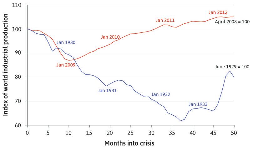
The Great Depression and the global financial crisis: Industrial production.
Figure 17.1a The Great Depression and the global financial crisis: Industrial production.
Miguel Almunia, Agustín Bénétrix, Barry Eichengreen, Kevin H. O’Rourke, and Gisela Rua. 2010. ‘From Great Depression to Great Credit Crisis: Similarities, Differences and Lessons.’ Economic Policy 25 (62): pp. 219–65. Updated using CPB Netherlands Bureau for Economic Policy Analysis. 2015. ‘World Trade Monitor.’
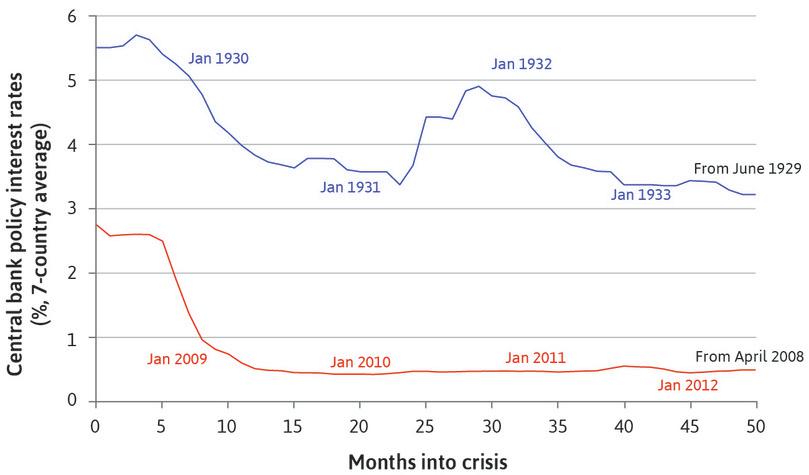
The Great Depression and the global financial crisis: Monetary policy.
Figure 17.1b The Great Depression and the global financial crisis: Monetary policy.
As in Figure 17.1a, updated using national central bank data.
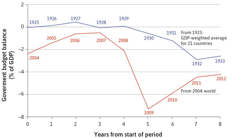
The Great Depression and the global financial crisis: Fiscal policy.
Figure 17.1c The Great Depression and the global financial crisis: Fiscal policy.
As in Figure 17.1a, updated using International Monetary Fund. 2009. World Economic Outlook: January 2009; International Monetary Fund. 2013. ‘IMF Fiscal Monitor April 2013: Fiscal Adjustment in an Uncertain World, April 2013.’ April 16.
17.1 Three economic epochs
In the past 100 years, the economies we often refer to as ‘advanced’ (basically meaning ‘rich’), including the US, western Europe, Australia, Canada, and New Zealand, have seen average living standards measured by output per capita grow six-fold. Over the same period, hours of work have fallen. This is a remarkable economic success, but it has not been a smooth ride.
- aggregate demand
- The total of the components of spending in the economy, added to get GDP: Y = C + I + G + X – M. It is the total amount of demand for (or expenditure on) goods and services produced in the economy. See also: consumption, investment, government spending, exports, imports.
- supply side (aggregate economy)
- How labour and capital are used to produce goods and services. It uses the labour market model (also referred to as the wage-setting curve and price-setting curve model). See also: demand side (aggregate economy).
- great moderation
- Period of low volatility in aggregate output in advanced economies between the 1980s and the 2008 financial crisis. The name was suggested by James Stock and Mark Watson, the economists, and popularized by Ben Bernanke, then chairman of the Federal Reserve.
Units 1 and 2 told the story of how rapid growth began. In Figures 13.2 and 13.3, we contrasted the steady long-run growth rate from 1921 to 2011 with the fluctuations of the business cycle, which go from peak to peak every three to five years.
In this unit we will study three distinctive epochs. Each begins with a period of good years (the light shading in Figure 17.2), followed by a period of bad years (the dark shading):
- 1921 to 1941: The crisis of the Great Depression is the defining feature of the first epoch. It inspired Keynes’ concept of aggregate demand, now standard in economics teaching and policymaking.
- 1948 to 1979: The golden age epoch stretched from the end of the Second World War to 1979, and is named for the economic success of the 1950s and 1960s. The golden age ended in the 1970s with a crisis of profitability and productivity, and the emphasis in economics teaching and policymaking shifted away from the role of aggregate demand toward supply-side problems, such as productivity and decisions by firms to enter and exit markets.
- 1979 to 2015: In the most recent epoch, the global financial crisis caught the world by surprise. The potential of a debt-fuelled boom to cause havoc was neglected during the preceding years of stable growth and seemingly successful macroeconomic management, which had been called the great moderation.
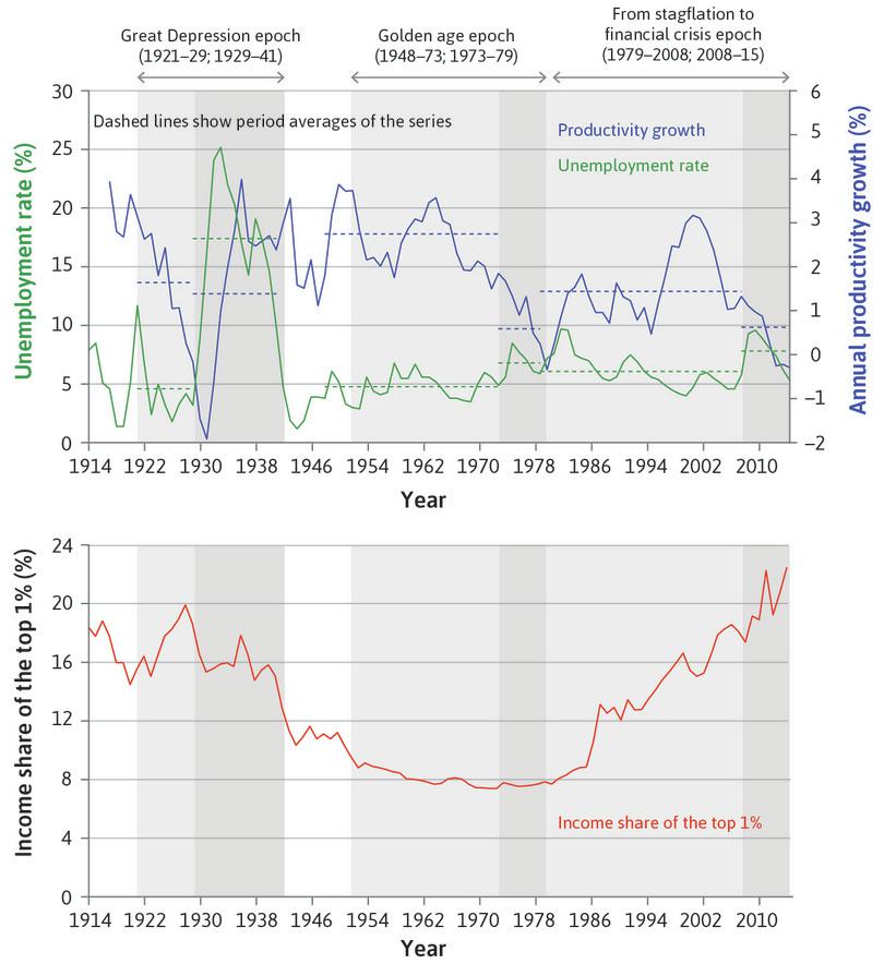
Unemployment, productivity growth, and inequality in the US (1914–2015).
Figure 17.2 Unemployment, productivity growth, and inequality in the US (1914–2015).
United States Bureau of the Census. 2003. Historical Statistics of the United States: Colonial Times to 1970, Part 1. United States: United States Govt Printing Office; Facundo Alvaredo, Anthony B Atkinson, Thomas Piketty, Emmanuel Saez, and Gabriel Zucman. 2016. ‘The World Wealth and Income Database (WID).’; US Bureau of Labor Statistics; US Bureau of Economic Analysis.
The term ‘crisis’ is routinely applied to the first and the last of these episodes because they represented an unusual but recurrent cataclysmic divergence from the normal ups-and-downs of the economy. In the second epoch, the end of the golden age also marked a sharp deviation from what had become normal. The three unhappy surprises that ended the epochs are different in many respects, but they share a common feature: positive feedbacks magnified the effects of routine shocks that would have been dampened under other circumstances.
What does Figure 17.2 show?
- Productivity growth: A broad measure of economic performance is the growth of hourly productivity in the business sector. Productivity growth hit low points in the Great Depression, at the end of the golden age epoch in 1979, and in the wake of the financial crisis. The golden age of capitalism got its name due to the extraordinary productivity growth until late in that epoch. The dashed blue lines show the average growth of productivity for each sub-period.
- Unemployment: High unemployment, shown in red, dominated the first epoch. The success of the golden age was marked by low unemployment as well as high productivity growth. The end of the golden age produced spikes in unemployment in the mid 1970s and early 1980s. In the third epoch, unemployment was lower at each successive business cycle trough until the financial crisis, when high unemployment re-emerged.
- Inequality: Figure 17.2 also presents data on inequality for the US: the income share of the top 1%. The richest 1% had nearly one-fifth of income in the late 1920s just before the Great Depression. Their share then steadily declined until a U-turn at the end of the golden age eventually restored the income share of the very rich to 1920s levels.
We saw in earlier units that continuous technological progress has characterized capitalist economies, driven by the incentives to introduce new technology. Based on their expected after-tax profits, entrepreneurs make investment decisions to get a step ahead of their competitors. Productivity growth reflects their collective decisions to invest in new machinery and equipment that embody improvements in technology. Figure 17.3 shows the growth rate of the capital stock and the profit rate of firms in the non-financial corporate sector of the US economy (before and after the payment of taxes on profits).
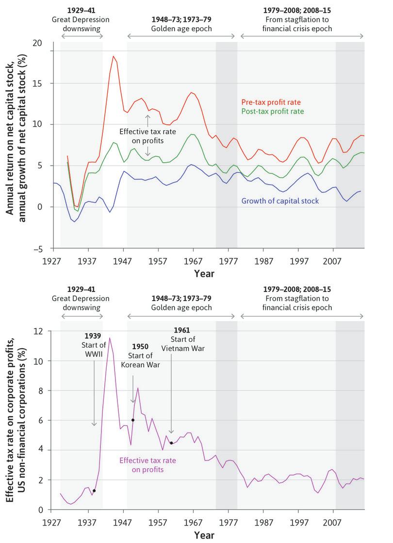
Upper panel: Capital stock growth and profit rates for US non-financial corporations (1927–2015). Lower panel: Effective tax rate on profits for US non-financial corporations (1929–2015).
Figure 17.3 Upper panel: Capital stock growth and profit rates for US non-financial corporations (1927–2015). Lower panel: Effective tax rate on profits for US non-financial corporations (1929–2015).
The data in Figure 17.3 illustrates that capital stock growth and firm profitability tend to rise and fall together. As we saw in Unit 14, investment is a function of expected post-tax profits, and expectations will be influenced by what has happened to profitability in the recent past. Once firms make a decision to invest, there is a lag before the new capital stock is ordered and installed.
- effective tax rate on profits
- This is calculated by taking the before-tax profit rate, subtracting the after-tax profit rate, and dividing the result by the before-tax profit rate. This fraction is usually multiplied by 100 and reported as a percentage.
As profitability was restored following the collapse of the stock market in 1929 and the banking crises of 1929–31, investment recovered and the capital stock began to grow again. During the golden age, profitability and investment were both buoyant. A closer look at Figure 17.3 is revealing. Investment depends on post-tax profitability and we can see that the gap between the pre-tax (red) and post-tax (green) rate of profit declined during the golden age. The lower panel shows the effective tax rate on corporate profits.
Wars have to be financed, and the tax on businesses increased during the Second World War and the Korean War, and more slowly over the course of the Vietnam War. The effective tax rate on profits fell from 8% to 2% during the 30 years from the early 1950s. This helped to stabilize the post-tax rate of profit. In the late 1970s and early 1980s, taxes on profits were cut sharply. Thereafter the pre-tax profit rate fluctuated without a trend. But in spite of the stabilization of profitability in the third epoch, the growth rate of the capital stock fell.
On the eve of the financial crisis, Figures 17.2 and 17.3 show that the richest Americans were doing very well. But this did not stimulate investment, with the capital stock growing more slowly than at any time since the Second World War. The onset of the financial crisis also coincided with a peak in private sector debt (shown in Figure 17.4). Debt in financial firms and in households was at a postwar high (relative to the size of GDP). The swelling in the amount of debt was clearest for financial firms, but households also increased their debt-to-GDP ratio steadily through the 2000s.
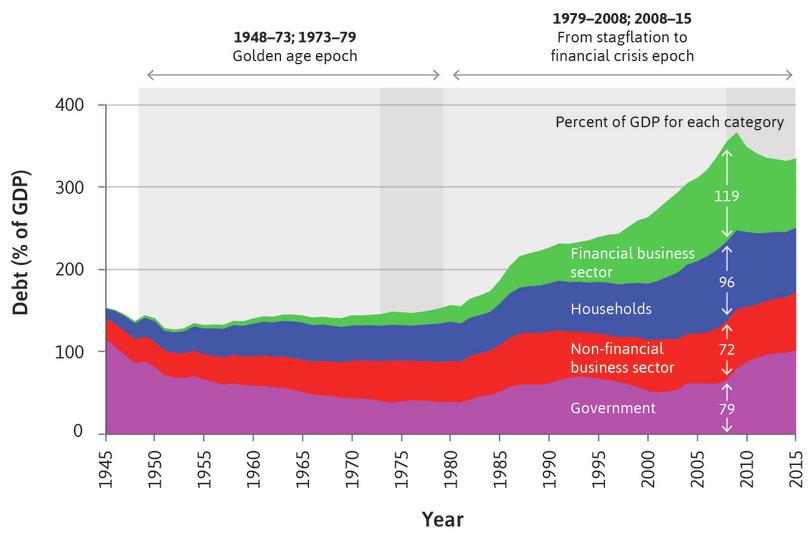
Debt as a percentage of GDP in the US: Households, non-financial business sector, financial business sector, and the government (1945–2015).
Figure 17.4 Debt as a percentage of GDP in the US: Households, non-financial business sector, financial business sector, and the government (1945–2015).
US Federal Reserve. 2016. ‘Financial Accounts of the United States, Historical.’ December 10; US Bureau of Economic Analysis.
Figure 17.5a summarizes the key features of each period in the US economy over the past century.
| Name of Period | Dates | Important features of the US economy |
|---|---|---|
| 1920s | 1921–1929 | Low unemployment High productivity growth Rising inequality |
| Great Depression | 1929–1941 | High unemployment Falling prices Unusually low growth rate of business capital stock Falling inequality |
| Golden age | 1948–1973 | Low unemployment Unusually high productivity growth Unusually high growth rate of capital stock Falling effective tax rate on corporate profits Falling inequality |
| Stagflation | 1973–1979 | High unemployment and inflation Low productivity growth Lower profits |
| 1980s and the great moderation | 1979–2008 | Low unemployment and inflation Falling growth rate of business capital stock Sharply rising inequality Rising indebtedness of households and banks |
| Financial crisis | 2008–2015 | High unemployment Low inflation Rising inequality |
The performance of the US economy over a century.
Figure 17.5a The performance of the US economy over a century.
The three epochs of modern capitalism were worldwide phenomena, but some countries experienced them differently compared to the US. By 1921, the US had been the world productivity leader for a decade, and the world’s largest economy for 50 years. Its global leadership in technology and its global firms help explain rapid catch-up growth in Europe and Japan during the golden age. On either side of the golden age, the crises that began in the US in 1929 and 2008 became global crises. Figure 17.5b summarizes important differences between the US and other rich countries.
| Name of Period | Differences between US and other rich countries |
|---|---|
| Great Depression | US: Large, sustained downturn in GDP starting from 1929 UK: Avoided a banking crisis, experienced a modest fall in GDP |
| Golden age | US: Technology leader Outside US: Diffusion of technology creates catch-up growth, improving productivity |
| Financial crisis | US: Housing bubble creates banking crisis Germany, Nordic countries, Japan, Canada, Australia: Did not experience bubble, largely avoided financial crisis |
| International openness (all three periods) | More important in most countries than in the US |
A cross-national comparison of the Great Depression, the golden age, and the financial crisis: Distinctive features of the US.
Figure 17.5b A cross-national comparison of the Great Depression, the golden age, and the financial crisis: Distinctive features of the US.
The three epochs of modern capitalism are very different, as Figures 17.5a and 17.5b show. We need to use the full range of tools of analysis we have developed in previous units to understand their dynamics, and how one epoch is related to another.
Question 17.1 Choose the correct answer(s)
The following figure shows the unemployment rate (left-hand axis) and productivity growth (right-hand axis) in the US between 1914 and 2015.
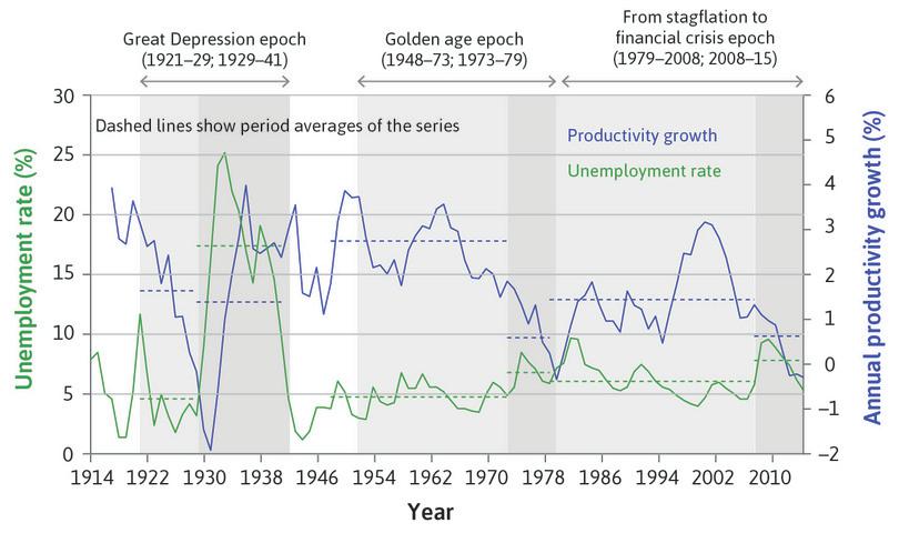
Based on this information, which of the following statements is correct?
- The average unemployment rates in the boom years of the first two epochs were below 5%, while that in the 1979–2008 period was around 6%.
- Productivity growth fell very sharply at the onset of the Great Depression. However it also rebounded sharply, making the average productivity growth for the era about 2%, very similar to the average productivity growth of the 1979–2008 growth years.
- The average unemployment rates in the boom years of the first two epochs were below 5%, while the average productivity growth rates were around 2.2% and 3.2% respectively. Over the 1979–2008 period, the average unemployment rate was around 6% while the average productivity growth rate was 2.1%.
- The unemployment rate almost reached 10% in the early 1980s, higher than the peak hit during the financial crisis period.
Question 17.2 Choose the correct answer(s)
The following figure shows the income share of the top 1% richest households in the US between 1914 and 2013.
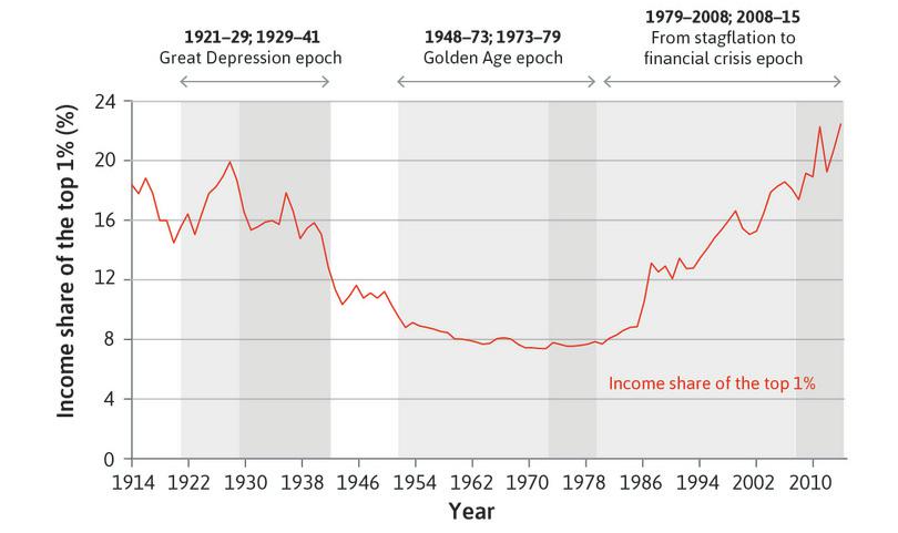
Based on this information, which of the following statements are correct?
- This is not true. For example, the share of top 1% fell consistently during the golden Age of 1948–73.
- Inequality had years of decline and years of increase in both the Great Depression and the recession after the financial crisis.
- Inequality also rose in the boom years of the 1920s. The golden age was distinct in that inequality fell consistently during the period.
- They received 19% of total income.
17.2 The Great Depression, positive feedbacks, and aggregate demand
Capitalism is a dynamic economic system, and as we saw in Unit 13, booms and recessions are a recurrent feature even when weather-driven fluctuations in agricultural output are of limited importance in the economy. But not all recessions are equal. In Unit 14, we saw that in 1929 a downturn in the US business cycle similar to others in the preceding decade transformed into a large-scale economic disaster—the Great Depression.
The story of how the Great Depression happened is dramatic to us, and must have been terrifying to those who experienced it. Small causes led to ever-larger effects in a downward spiral, like the cascading failures of an electricity grid during a blackout. Three simultaneous positive feedback mechanisms brought the American economy down in the 1930s:
- Pessimism about the future: The impact of a decline in investment on unemployment and of the stock market crash of 1929 on future prospects spread fear among households. They prepared for the worst by saving more, bringing about a further decline in consumption demand.
- Failure of the banking system: The resulting decline in income meant that loans could not be repaid. By 1933, almost half of the banks in the US had failed, and access to credit shrank. The banks that did not fail raised interest rates as a hedge against risk, further discouraging firms from investing and curbing household spending on automobiles, refrigerators, and other durable goods.
- Deflation: Prices fell as unsold goods piled up on store shelves.
- deflation
- A decrease in the general price level. See also: inflation.
Deflation affects aggregate demand through several routes. The most important channel operated through the effect of deflation on those with high debts. Since debts were denominated in nominal terms, deflation pushed up their real value. This positive feedback channel was new because in earlier episodes of deflation levels of debt had been much lower. Households stopped buying cars and houses, and many debtors become insolvent, creating problems for both borrowers and the banks. One-fifth of those in owner-occupied and rented accommodation were in default. Farmers were among those with high levels of debt. Prices of their produce were falling, pulling down their incomes directly and pushing up the burden of their debt. They responded to this by increasing production, which made the situation worse by reducing prices further. When prices are falling, people also postpone the purchase of durables, which further reduces aggregate demand.
Few people understood these positive feedback mechanisms at the time, and the government’s initial attempts to reverse the downward spiral failed. This was partly because the government’s actions were based on mistaken economic ideas. It was also because even if they had pursued ideal policies, the government’s share of the economy was too small to counter the powerful destabilizing trends in the private sector.
Figure 17.6 shows the fall in industrial production that started in 1929. In 1932 it was less than 60% of the 1929 level. This was followed by a recovery, until it fell again by 20% in 1937. Unemployment remained above 10% until 1941, the year the US entered the Second World War. Consumer prices fell with GDP from 1929 to 1933 and remained stable until the early 1940s.
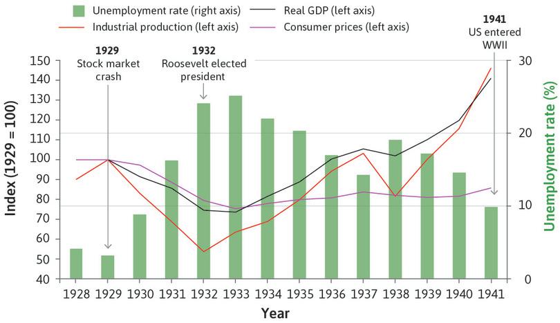
The effect of the Great Depression on the US economy (1928–1941).
Figure 17.6 The effect of the Great Depression on the US economy (1928–1941).
United States Bureau of the Census. 2003. [Historical Statistics of the United States: Colonial Times to 1970, Part 1] (tinyco.re/9147417). United States: United States Govt Printing Office; Federal Reserve Bank of St Louis (FRED).
Exercise 17.1 Farmers in the Great Depression
During the Great Depression, demand for agricultural output fell. Faced with falling prices for agricultural output and with high levels of debt, farmers increased production. The response of farmers may have made sense from an individual point of view, but collectively it made the situation worse. Using wheat farmers as an example, and assuming that wheat farms are all identical, draw diagrams of an individual price-taking farm’s cost curves and industry-wide supply and demand to illustrate this situation. Explain your reasoning.
17.3 Policymakers in the Great Depression
Just as the day of Australia’s major bushfire is now called Black Saturday, the day that the Great Depression started is now known as Black Thursday. On Thursday 24 October 1929, the US Dow Jones Industrial Average fell 11% on opening, starting three years of decline for the US stock market. Figure 17.7 shows the business cycle upswings and downswings from 1924 to 1941.
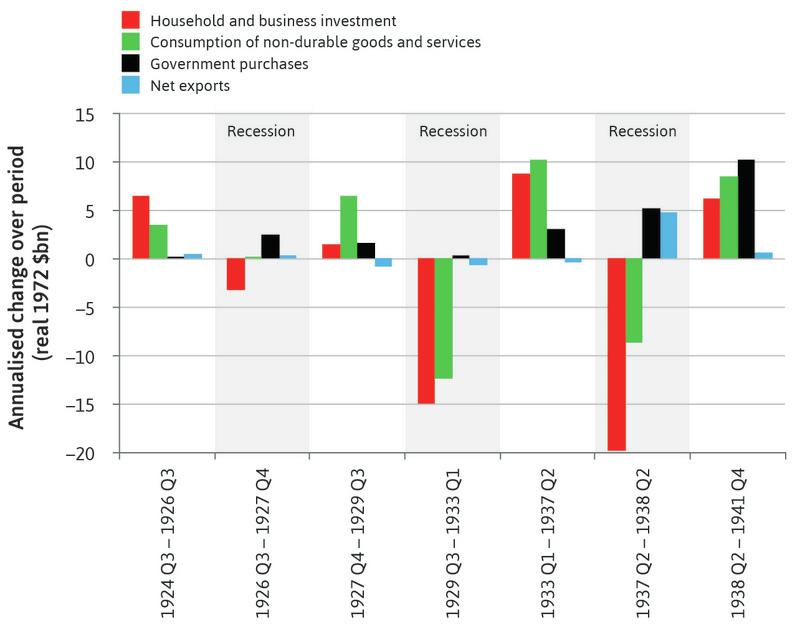
Changes in the components of aggregate demand during upswings and downswings (1924 Q3 to 1941 Q4).
Figure 17.7 Changes in the components of aggregate demand during upswings and downswings (1924 Q3–1941 Q4).
Appendix B in Robert J. Gordon. 1986. The American Business Cycle: Continuity and Change. Chicago, Il: University of Chicago Press.
The long downswing from the third quarter of 1929 until the first quarter of 1933 was driven by big falls in household and business investment (the red bar), and in consumption of non-durables (the green bar). Recall that in Figure 14.6 we used the multiplier model to describe how this shock created a fall in aggregate demand, and in Figure 14.8 we described a model of how households had cut consumption to restore their target wealth, to understand the observed behaviour of households and firms in the Great Depression.
In Unit 14, we showed how government policy could amplify or dampen fluctuations. In the opening years of the Great Depression, government policy both amplified and prolonged the shock. Initially, government purchases and net exports hardly changed. As late as April 1932 President Herbert Hoover told Congress that ‘far-reaching reduction of governmental expenditures’ was necessary, and advocated a balanced budget. Hoover was replaced by Franklin Delano Roosevelt in 1932, at which point government policy changed.
Fiscal policy in the Great Depression
Fiscal policy made little contribution to recovery until the early 1940s. Estimates suggest that output was 20% below the full employment level in 1931, for example, which means that the small budget surplus in that year would have implied a large cyclically adjusted surplus, given the decline in tax revenues in the depressed economy.
Under Roosevelt, from 1932 to 1936 the government ran deficits. When the economy went into recession in 1938–39, the deficit shrank from its peak of 5.3% in 1936 to 3% in 1938. This was another mistake that reinforced the downturn. The big increase in military spending from early 1940 (well before the US entered the Second World War in late 1941) contributed to the recovery.
Monetary policy in the Great Depression
Monetary policy prolonged the Great Depression. The real interest rate data in Figure 17.8 suggest that monetary policy was contractionary in the US economy from 1925 onwards: the real interest rate increased, reaching a peak of 13% in 1932. Once the downturn began in 1929, this policy stance reinforced, rather than offset, the decline of aggregate demand. But note that the nominal interest rate was falling after its peak in 1929; the real interest rate went up because prices were falling too. Interest-sensitive spending on buildings and consumer durables decreased sharply.
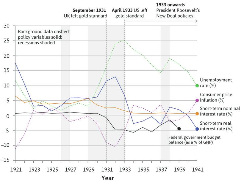
Policy choices in the Great Depression: The US (1921–1941).
Figure 17.8 Policy choices in the Great Depression: The US (1921–1941).
Milton Friedman and Anna Jacobson J. Schwartz. 1982. Monetary Trends in the United States and the United Kingdom, Their Relation to Income, Prices, and Interest Rates, 1867–1975. Chicago, Il: University of Chicago Press; United States Bureau of the Census. 2003. Historical Statistics of the United States: Colonial Times to 1970, Part 1. United States: United States Govt Printing Office; Federal Reserve Bank of St Louis (FRED).
The gold standard
- gold standard
- The system of fixed exchange rates, abandoned in the Great Depression, by which the value of a currency was defined in terms of gold, for which the currency could be exchanged. See also: Great Depression.
- zero lower bound
- This refers to the fact that the nominal interest rate cannot be negative, thus setting a floor on the nominal interest rate that can be set by the central bank at zero. See also: quantitative easing.
The US was still on what was known as the gold standard. This meant that the US authorities promised to exchange dollars for a specific quantity of gold (the promise was to pay an ounce of gold for $20.67). Under the gold standard, the authorities had to continue to pay out gold at the fixed rate and, if there was a fall in demand for US dollars, gold would flow out of the country. To prevent this, either the country’s tradable goods had to become more competitive (boosting gold inflows through higher net exports) or gold had to be attracted through capital inflows. This could done by either putting up the nominal interest rate or keeping it high relative to the interest rate in other countries. To avoid contributing to the gold outflow, policymakers were reluctant to push the interest rate down to the zero lower bound. This closed off the possibility of using monetary policy to counteract the recession.
Unless wages decline rapidly to raise international competitiveness and boost the inflow of gold through higher exports and lower imports, sticking to the gold standard in a recession is destabilizing, as it will amplify the downturn. There was a very large outflow of gold from the US after the UK left the gold standard in September 1931. One reason for speculation against the US dollar (that is, investors selling dollars for gold) was that there were expectations that the US would also abandon the gold standard and devalue the dollar. If it did, those holding dollars would lose.
A change in expectations
In 1933 Roosevelt began a program of changes to economic policy:
- New Deal
- US President Franklin Roosevelt’s program, begun in 1933, of emergency public works and relief programs to employ millions of people. It established the basic structures for modern state social welfare programs, labour policies, and regulation.
- The New Deal: This committed federal government spending to a range of programs to increase aggregate demand.
- The US left the gold standard: In April 1933 the US dollar was devalued to $35 per ounce of gold, and the nominal interest rate was reduced to close to the zero lower bound (see Figure 17.8).
- Roosevelt also introduced reforms to the banking system: This followed bank runs in 1932 and early 1933.
The change in people’s beliefs about the future was just as important as these policy changes. On 4 March 1933, in his inaugural address as president, Roosevelt had told Americans that: ‘the only thing we have to fear is fear itself—nameless, unreasoning, unjustified terror’.
The Great Depression
The period during the 1930s in which there was a sharp fall in output and employment, experienced in many countries.
- Countries that left the gold standard earlier in the 1930s recovered earlier.
- In the US, Roosevelt’s New Deal policies accelerated recovery from the Great Depression, partly by causing a change in expectations.
We have seen that the terrors of consumers and investors in 1929 had been justified. But due to a combination of Roosevelt’s New Deal policies and early signs of recovery that were already present before he became president, households and firms began to think that prices would stop falling and that employment would expand.
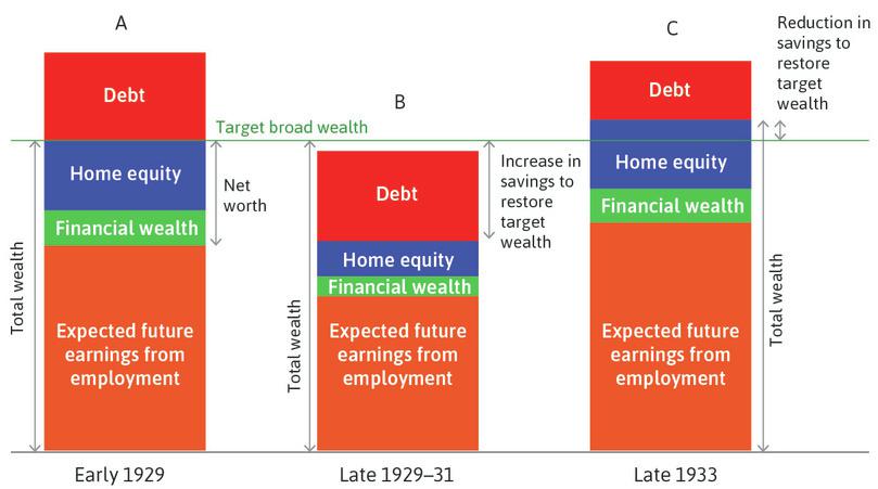
The Great Depression and recovery: Households cut consumption to restore target wealth in the depression; and increased consumption from 1933.
Figure 17.9 The Great Depression and recovery: Households cut consumption to restore target wealth in the depression; and increased consumption from 1933.
Figure 17.9 adds a third column to the model of household wealth that we first encountered in Figure 14.8. Column C shows the household’s perspective from late 1933. By that time, output and employment were growing. With much of the uncertainty about the future resolved, households re-evaluated their expected wealth (including their expected earnings from employment). They reversed the cutbacks in consumption because they saw no need to make additional savings. To the extent that they now expected their income prospects and asset prices to return to pre-crisis levels, consumption would be restored. Any increase in wealth above target due to the increased savings during the Great Depression years (shown by wealth above target in column C) would create an additional boost to consumption.
The slow path to recovery had begun. But the US economy would not return to pre-Great Depression levels of employment until Roosevelt was in his third term as president and the Second World War had begun.
Exercise 17.2 Advantages and disadvantages of fixed exchange rates
In an ‘Economist in action’ video, Barry Eichengreen, an economist and economic historian, discusses fixed exchange rate systems such as the gold standard in the Great Depression and the euro system in the aftermath of the financial crisis.
- According to the video, what are some advantages and disadvantages of fixed exchange rate systems?
- How can countries that are in these exchange rate systems effectively respond to economic shocks? What are some features of the euro system that make it difficult to respond effectively?
Question 17.3 Choose the correct answer(s)
Franklin Roosevelt became the US President in 1933. In the period after he became the president:
- The federal government deficit increased to 5.6% of GNP in 1934.
- The short-term nominal interest rate fell from 1.7% in 1933 to 0.75% in 1935.
- The CPI fell by 5.2% in 1933 and rose by 3.5% in 1934.
- The US left the gold standard in April 1933.
- The New Deal was launched in 1933 and included proposals to increase federal government spending in a wide range of programs and reforms to the banking system.
Which of the following statements is correct regarding the years immediately after Roosevelt became the US president?
- More optimistic expectations lead to increased consumer spending, as shown in Figure 17.9.
- The abandonment of the gold standard meant that the US dollar could be devalued, (from $20.67 to $35 per ounce of gold). It was no longer necessary to keep the interest rate high to maintain the dollar at the higher rate (meaning fewer dollars per ounce).
- With the nominal interest rate falling, and with inflation turning positive from negative, the real interest rate fell sharply (and became negative in 1934).
- Increased government deficit means fiscal expansion.
17.4 The golden age of high growth and low unemployment
The golden age of capitalism
The period of high productivity growth, high employment, and stable inflation extending from the end of the Second World War to the early 1970s.
- The gold standard was replaced by the more flexible Bretton Woods system.
- Employers and employees shared the benefits of technological progress, thanks to the postwar accord.
- The golden age ended with a period of stagflation in the 1970s.
The years from 1948 until 1973 were remarkable in the history of capitalism. In the US, we saw in Figure 17.2 that productivity growth was more rapid and unemployment was lower than in the other periods. But this 25-year golden age of capitalism was not confined to the US. Japan, Australia, Canada, New Zealand, and countries across western Europe experienced a golden age as well. Unemployment rates were historically low (see Figure 16.1). Figure 17.10 shows data from 1820 to 1913 for 13 advanced countries, and for 16 countries from 1950 to 1973.
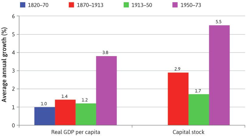
The golden age of capitalism in historical perspective.
Figure 17.10 The golden age of capitalism in historical perspective.
Table 2.1 in Andrew Glyn, Alan Hughes, Alain Lipietz, and Ajit Singh. 1989. ‘The Rise and Fall of the Golden Age’. In The Golden Age of Capitalism: Reinterpreting the Postwar Experience, edited by Stephen A. Marglin and Juliet Schor. New York, NY: Oxford University Press. Data from 1820 to 1913 for 13 advanced countries, and for 16 countries from 1950.
The growth rate of GDP per capita was more than two-and-a-half times as high during the golden age as in any other period. Instead of doubling every 50 years, living standards were doubling every 20 years. The importance of saving and investment is highlighted in the right panel, where we can see that the capital stock grew almost twice as fast during the golden age as it did between 1870 and 1913.
Figure 17.11 shows the story of how western European countries and Japan (almost) caught up to the US. In this figure, the level of GDP per hour worked in the US is set at the level of 100 throughout, and so the figure tells us nothing about the performance of the US itself (we have to use Figure 17.2 for that). However, it is a striking way to represent the starting point of economies relative to the US immediately after the Second World War and their trajectories in the years that followed. This was known as catch-up growth.
- catch-up growth
- The process by which many (but far from all) economies in the world close the gap between the world leader and their own economy.
The three large defeated countries (Germany, Italy, and Japan) were furthest behind in 1950. Japan’s GDP per hour worked was less than one-fifth the level of the US. Clearly, growth of all of these economies was faster than the US during the golden age: all moved much closer to the level of US productivity.
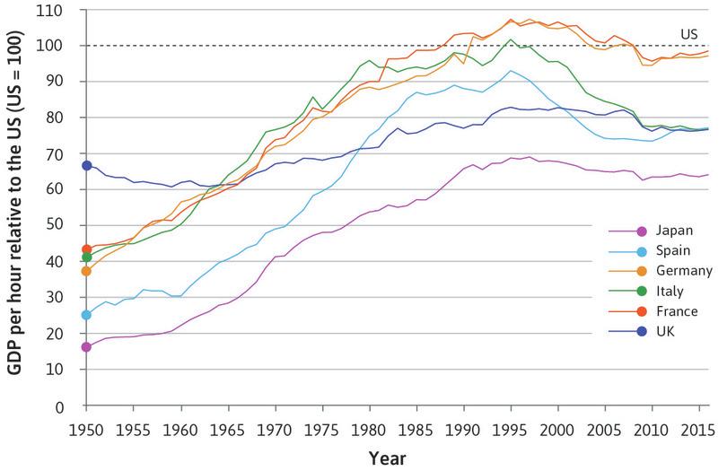
Catching up to the US during the golden age and beyond (1950–2016).
Figure 17.11 Catching up to the US during the golden age and beyond (1950–2016).
The Conference Board. 2016. ‘Total Economy Database.’
What was the secret of golden age performance in the productivity leader (the US) and in the follower countries?
- Changes in economic policymaking and regulation: These resolved the problems of instability that characterized the Great Depression.
- New institutional arrangements between employers and workers: These created conditions in which it was profitable for firms to innovate. In the US, the technology leader, this meant new technologies, while the follower countries often adopted improved technology and management already in use in the US. Because trade unions and workers’ political parties were now in a stronger position to bargain for a share of the productivity gains, they supported innovation—even when it meant temporary job destruction.
After the Second World War, governments had learned the lessons of the Great Depression. This affected national and international policymaking. Just as Roosevelt’s New Deal signalled a new policy regime and raised expectations in the private sector, postwar governments provided reassurance that policy would be used to support aggregate demand if necessary.
Postwar governments were larger in all of these countries and grew throughout the 1950s and 1960s. Figure 14.1 showed the decline in output fluctuations after 1950, and the much larger size of government in the US. In Unit 14, we saw how a larger government provides more automatic stabilization for the economy. The modern welfare state was built in the 1950s, and unemployment benefits were introduced. This also formed part of the automatic stabilization.
- Bretton Woods system
- An international monetary system of fixed but adjustable exchange rates, established at the end of the Second World War. It replaced the gold standard that was abandoned during the Great Depression.
Given the cost of adherence to the gold standard during the Great Depression, it was clear that a new policy regime for international economic relations had to be put in place. The new regime was called the Bretton Woods system. It was named after the ski resort in New Hampshire where representatives of the major economies, including Keynes, created a system of rules that was more flexible than the gold standard. Exchange rates were tied to the US dollar rather than gold, and if countries became very uncompetitive—if they faced a ‘fundamental disequilibrium’ in external accounts, in the words of the agreement—devaluations of the exchange rate were permitted. When a currency like the British pound was devalued (as occurred in November 1967) it became cheaper to buy pounds. This boosted the demand for British exports and reduced the demand of British residents for goods produced abroad. The Bretton Woods system worked fairly well for most of the golden age.
17.5 Workers and employers in the golden age
High investment, rapid productivity growth, rising wages, and low unemployment defined the golden age. How did this virtuous circle work?
- After-tax profits in the US economy remained high: This persisted from the end of the Second World War through the 1960s (look again at Figure 17.3), and the situation was similar in other advanced economies.
- Profits led to investment: The widespread expectation that high profits would continue in the future provided the conditions for sustained high levels of investment (refer back to the model of investment spending in Section 14.4).
- High investment and continued technological progress created more jobs: Unemployment stayed low.
- The power of workers: Trade unions and political movements allied with employees were sufficiently strong to secure sustained increases in wages. But accords between unions and employers meant that unions tended to act in an inclusive manner (Unit 16), and sustained the union voice effect (Unit 9), encouraging cooperation between workers and firms in the face of new technology adoption.
Follow the steps in the analysis in Figure 17.12 to see how these four bullet points explaining the golden age can be translated into shifts in the price-setting curve and the wage-setting curve. Recall from Unit 16 that the price-setting curve shows the real wage consistent with employers maintaining investment at a level that keeps employment constant. This means that a real wage below the price-setting curve will encourage firms to enter or raise their investment, and employment rises.

The golden age: Using the wage- and price-setting curves.
Figure 17.12 The golden age: Using the wage- and price-setting curves.
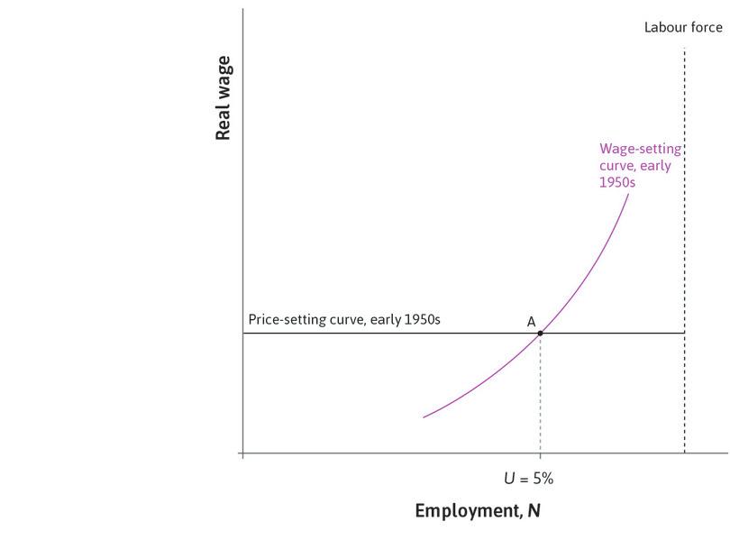
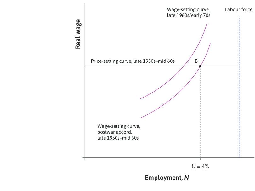
The beginning of the golden age
Suppose that the US economy was at point A at the beginning of the golden age, with unemployment of 5%.
Figure 17.12a Suppose that the US economy was at point A at the beginning of the golden age, with unemployment of 5%.
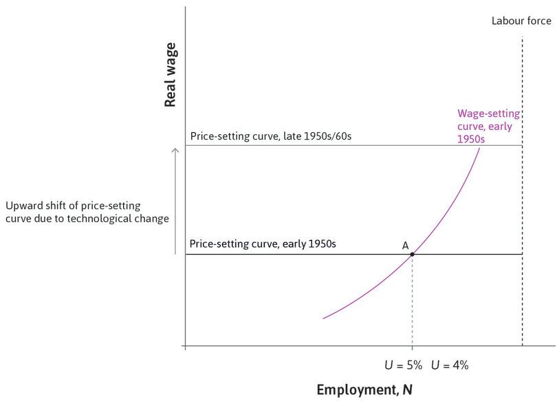
Technological progress
This shifts the price-setting curve up (to the one labelled ‘late 1950s/60s’). This stimulates high investment, consistent with the data for the growth of the capital stock in the US shown in Figure 17.3.
Figure 17.12b This shifts the price-setting curve up (to the one labelled ‘late 1950s/60s’). This stimulates high investment, consistent with the data for the growth of the capital stock in the US shown in Figure 17.3.
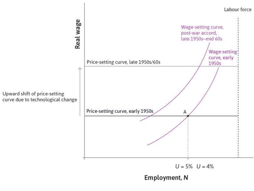
The wage-setting curve shifts up, but less than the price-setting curve
Strong unions and favourable government policies increased labour’s bargaining power. But through accords with employers, the resulting upward shift in the wage-setting curve was modest.
Figure 17.12c Strong unions and favourable government policies increased labour’s bargaining power. But through accords with employers, the resulting upward shift in the wage-setting curve was modest.
The actors agree
At point B, unions and employers agree about the scope for wage increases.
Figure 17.12d At point B, unions and employers agree about the scope for wage increases.
In the US, technological progress was rapid in the golden age as the innovations developed during the Great Depression and the Second World War were embodied in new capital equipment. The new technologies and new management techniques already in use in the US could also be used in the catch-up economies. In many of these countries golden age growth was even faster than at the technology frontier as defined by the US in Figure 17.11.
The strength of unions in wage-setting and the improvement in unemployment insurance during the 1950s and 60s are illustrated as an upward shift of the wage-setting curve in Figure 17.12. The outcome observed, with wages growing in line with productivity at low unemployment, is illustrated by point B.
Both trade unions and governments were important in this process. Between 1920 and 1933, trade unions in the US lost two-fifths of their members. During the 1930s, changes in the laws affecting trade unions, as well as the hardship of the Great Depression, reversed this decline. High demand for labour during the Second World War strengthened labour’s bargaining power, but trade union membership as a fraction of total employment peaked in the early 1950s. There was a subsequent steady decline during the next 50 years.
- postwar accord
- An informal agreement (taking different forms in different countries) among employers, governments, and trade unions that created the conditions for rapid economic growth in advanced economies from the late 1940s to the early 1970s. Trade unions accepted the basic institutions of the capitalist economy and did not resist technological change in return for low unemployment, tolerance of unions and other rights, and a rise in real incomes that matched rises in productivity.
Figure 17.13 shows both the growth of the government and the historically high level of trade union membership in the US. As we have seen, larger government partly reflected the new entitlements to unemployment benefits. In the wage- and price-setting curve model, higher unemployment benefits and stronger trade unions shift the wage-setting curve upwards, but when unions are inclusive and when there is a strong union voice effect, then this upwards shift is restrained.
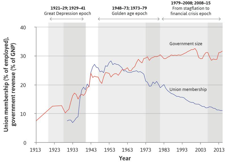
Trade union membership and the size of government in the US (1913–2015).
Figure 17.13 Trade union membership and the size of government in the US (1913–2015).
John Joseph Wallis. 2000. ‘American Government Finance in the Long Run: 1790 to 1990’. Journal of Economic Perspectives 14 (1): pp. 61–82; Gerald Mayer. 2004. Union Membership Trends in the United States. Washington, DC: Congressional Research Service; US Bureau of Economic Analysis.
Unions would tend to act in an inclusive manner, meaning that they refrained from using the full extent of their bargaining power (for example, in firms or plants where they had a very strong position). Instead, they cooperated in an economy-wide bargain designed to keep wage growth consistent with the constraint imposed by the price-setting curve. In return, employers would maintain investment at a level sufficient to keep unemployment low. This unwritten but widely observed pattern of sharing the gains to technological progress between employees and employers is termed the postwar accord.
These postwar accord relationships between employers, unions, and governments, which sustained high productivity growth, high real wage growth, and low unemployment, differed across countries. In Scandinavia, Austria, Belgium, Netherlands, Switzerland, and West Germany, wage-setting was either centralized in a single union, or coordinated among unions or employers’ associations, resulting in wage restraint. In technologically advanced sectors in France and Italy, governments intervened to set wages in dominant state-owned firms, creating wage guidance across the economy. The outcome was similar to the result in the countries with centralized wage-setting.
Where there was little cooperation between employers and unions, a country’s performance in the golden age was worse. In Figure 17.11, the UK’s relatively poor golden age performance shows up clearly. It started with higher productivity than the other large countries shown (that is, its productivity level in 1950 was the closest to that of the US) but was overtaken by France, Italy, and West Germany in the 1960s.
The British industrial relations system made an accord difficult. It combined very strong union power at the factory level with fragmented unions, which were unable to cooperate in the economy as a whole. The strength of local union shop stewards (representatives) in a system of multiple unions per plant led unions to attempt to outdo each other when negotiating wage deals, and created opposition to the introduction of new technology and new ways of organizing work.
The problems of the British economy were compounded because markets of British firms in former colonies were protected from competition, which weakened pressure to innovate. In the creative destruction process, competition creates incentives for firms to get a step ahead of their rivals and reduces the number of low-productivity firms. When competition is weak, existing firms and jobs are protected. The employers and workers in these firms share the monopoly rents, but the overall size of the pie is reduced because technological progress is slower.
In the US and the successful catch-up countries, postwar accords succeeded in creating the conditions for a high profit and high investment equilibrium. It delivered rapid productivity and real wage growth at low unemployment, but the British experience during the 1950s and 1960s (Figure 17.11) emphasizes that there is nothing automatic about achieving this outcome.
Question 17.4 Choose the correct answer(s)
Figure 17.12 describes the movements in employment, profits and wages in the 1950s to 1960s using the labour market model.
Which of the following statements is correct regarding this period?
- Persistent high profits since the end of the Second World War led to sustained high levels of investment, resulting in continuing technological progress.
- With workers cooperating to increase the size of the pie rather than claiming a larger share of the pie, the wage-setting curve’s rise was modest, allowing for high profits and investment.
- The golden age worked because workers had gained sufficient bargaining power to be confident that they could claim a substantial share in the mutual gains that technological progress made possible. Strong unions strengthened the union voice effect. Therefore they cooperated to increase the size of the pie (the postwar accord), leading to modest rises in the wage-setting curve.
- This virtuous cycle led to a rapidly rising price-setting curve, and a wage-setting curve that rose with it, but not faster.
17.6 The end of the golden age
- stagflation
- Persistent high inflation combined with high unemployment in a country’s economy.
The virtuous circle of the golden age began to break down in the late 1960s, in part as a result of its own successes. Years of low unemployment convinced workers that they had little chance of losing their jobs. Their demands for improvements in working conditions and higher wages drove down the profit rate. The postwar accord and its rationale of enlarging the pie gave way to a contest over the size of the slice that each group could get. This set the stage for the period of combined inflation and stagnation called stagflation that would follow.
Greater industrial strife in the late 1960s in leading economies signalled the breakdown of the golden age postwar accords. Figure 17.14 plots the days on strike per 1,000 industrial workers in advanced economies from 1950 to 2002. As strike activity peaked, wages measured relative to share prices increased rapidly. The postwar accords that helped create the golden age collapsed.
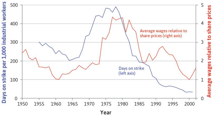
The end of the golden age: Strikes and wages relative to share prices in advanced economies (1950–2002).
Figure 17.14 The end of the golden age: Strikes and wages relative to share prices in advanced economies (1950–2002).
Andrew Glyn. 2006. Capitalism Unleashed: Finance, Globalization, and Welfare. Oxford: Oxford University Press.
Workers also demanded policies to redistribute income to the less well off and to provide more adequate social services, making it difficult for governments to run a budget surplus. In the US, additional military spending to fund the Vietnam War added to aggregate demand, keeping the economy at unsustainably high levels of employment.
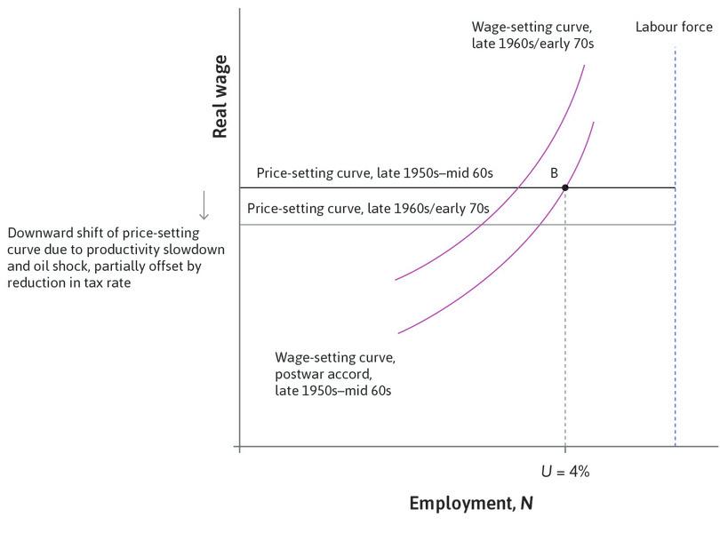
The process is represented in Figure 17.15 by an upward shift in the wage-setting curve (to the one labelled ‘late 1960s/early 70s’). At the same time, economy-wide productivity growth slowed (see Figure 17.2 for the US data). As the gap between the technology frontier in the US and in the catch-up countries in western Europe narrowed, it was more difficult to get easy gains from technology transfer (see Figure 17.11).
In 1973, the first oil price shock occurred. In Figure 17.15, this contributes to the downward shift of the price-setting curve (see the price-setting curve labelled ‘1973–79’ and refer back to Figure 15.11). Higher imported oil costs reduce the maximum real wage that workers can get if firms are to keep their profit margin unchanged.
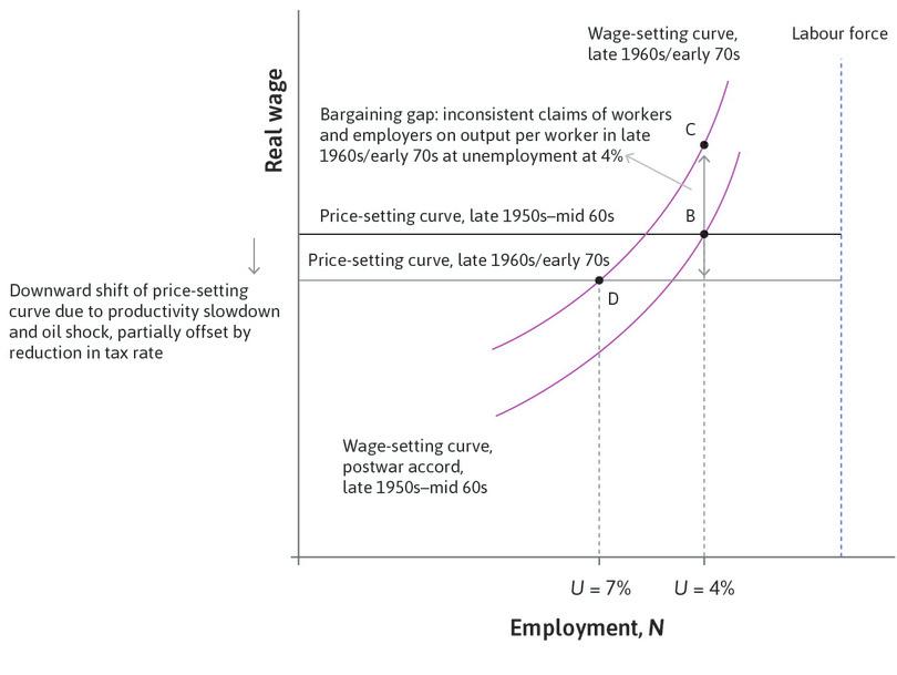
The end of the golden age: Using the wage and price-setting curves. (Note that the real wage on the vertical axis is measured post-tax and in terms of consumer prices.)
Figure 17.15 The end of the golden age: Using the wage and price-setting curves. (Note that the real wage on the vertical axis is measured post-tax and in terms of consumer prices.)
The postwar accord collapses
The upward shift in the wage-setting curve represents the collapse of postwar accords during the late 1960s and early 1970s.
Figure 17.15a The upward shift in the wage-setting curve represents the collapse of postwar accords during the late 1960s and early 1970s.
The first oil shock (1973)
In 1973, the first oil price shock occurred. This pushed the price-setting curve down.
Figure 17.15b In 1973, the first oil price shock occurred. This pushed the price-setting curve down.
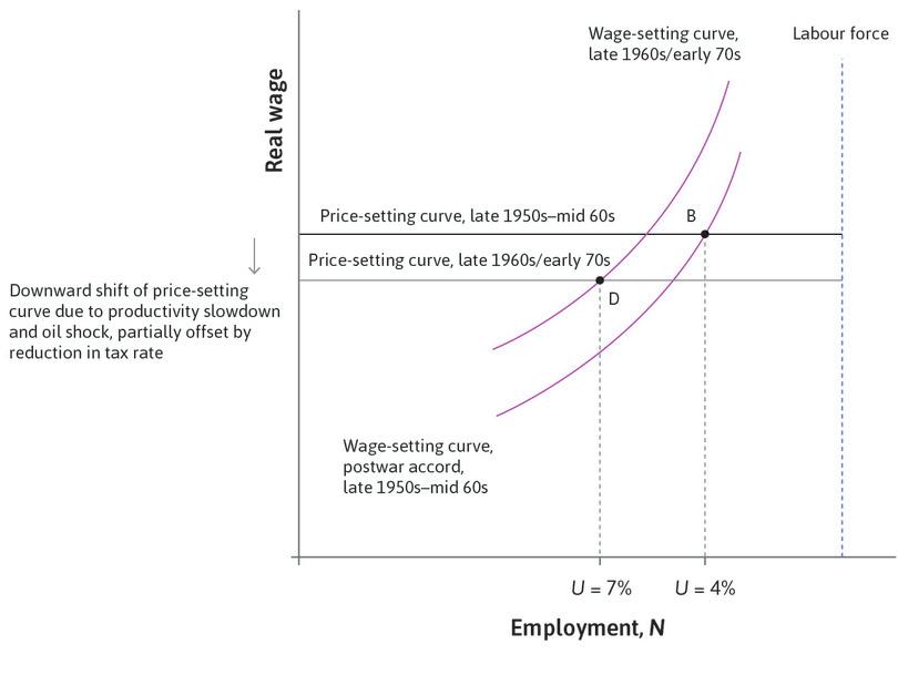
Inflation-stabilizing unemployment increases
The combination of a downward shift in the price-setting curve and an upward shift in the wage-setting curve meant that the sustainable long-term unemployment rate increased to 7%, shown at point D.
Figure 17.15c The combination of a downward shift in the price-setting curve and an upward shift in the wage-setting curve meant that the sustainable long-term unemployment rate increased to 7%, shown at point D.
A bargaining gap develops
The double-headed arrow at low unemployment shows the situation in the early 1970s.
Figure 17.15d The double-headed arrow at low unemployment shows the situation in the early 1970s.
What happened?
Wages did not rise to the level of point C. Under the impact of the upward pressure on wages and the oil price shock, the economy contracted and unemployment began to rise. But even a significant reduction in employment (short of increasing the unemployment rate to 7%) did not eliminate the bargaining gap shown in the figure. A result was an increase in the rate of inflation, as is shown in Figure 17.16.
Because of the strong bargaining position of workers in the early 1970s in most of the high-income economies, the oil price shock primarily hit employers, redistributing income from profits to wages (Figure 17.15). The era of fair-shares bargaining under the postwar accords was coming to a close.
- demand side (aggregate economy)
- How spending decisions generate demand for goods and services, and as a result, employment and output. It uses the multiplier model. See also: supply side (aggregate economy).
- supply side (aggregate economy)
- How labour and capital are used to produce goods and services. It uses the labour market model (also referred to as the wage-setting curve and price-setting curve model). See also: demand side (aggregate economy).
In the US and most of the high-income countries, unions were strong enough to defend their share of the pie even after the oil price increase and they chose to do so. In terms of the model, this meant wages were above the new price-setting curve. This cut into profits, so investment fell and the rate of productivity growth slowed. As predicted by the model in Figure 17.15, the outcome was rising inflation (Figure 17.16), falling profits (Figure 17.3), weak investment (Figure 17.3), and high unemployment (Figure 17.16).
In a handful of countries with inclusive and powerful trade unions (as described in Unit 16), the accord survived. In Sweden, for example, the powerful centralized labour movement restrained its wage claims to preserve profitability, investment, and high levels of employment (Figure 16.1).
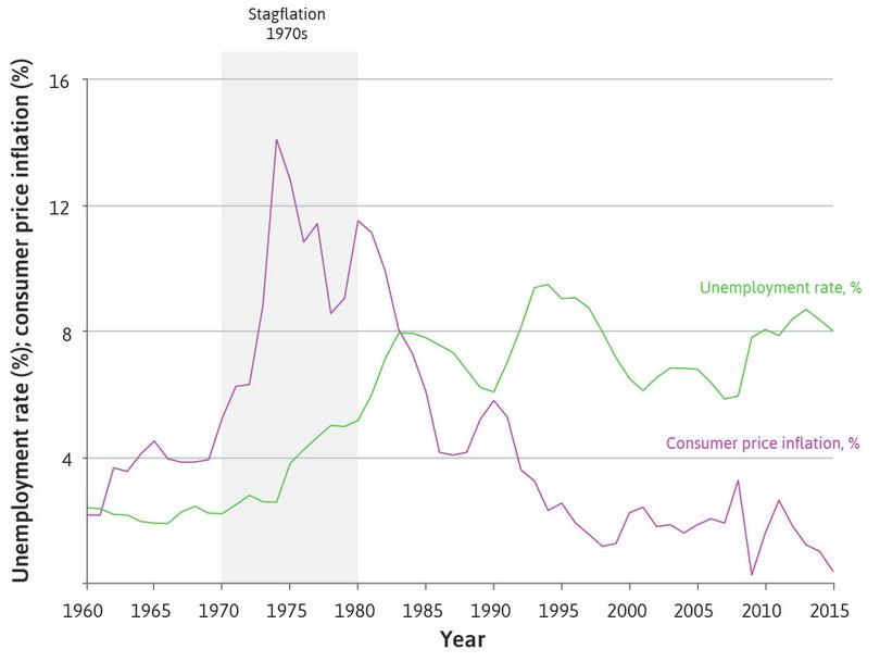
After the golden age: Unemployment and inflation in advanced economies (1960–2015).
Figure 17.16 After the golden age: Unemployment and inflation in advanced economies (1960–2015).
OECD. 2016. ‘OECD Statistics’.
The end of the golden age set off a new economic crisis, one that was very different from the Great Depression. The economic downturn of the 1930s had been propelled by problems of aggregate demand and for this reason it has been called a demand-side crisis. The end of the golden age has been called a supply-side crisis, because problems on the supply side of the economy depressed the profit rate, the rate of investment, and the rate of productivity growth.
The period that ensued came to be called stagflation because it combined high unemployment and high inflation. If the golden age was an unusual time during which everything went right at once, stagflation was an unusual time in which everything went wrong.
According to the Phillips curve model of Unit 15, inflation goes up when unemployment goes down; this is a movement along the Phillips curve. Figure 17.16 summarizes the unemployment and inflation data for the advanced economies from 1960–2013.
{:.show-page-number} shows the inflation and unemployment combinations for the US for each year between 1960 and 2014.](../images/web/figure-15-06-g.jpg)
Figure 15.6 shows the inflation and unemployment combinations for the US for each year between 1960 and 2014.
Just as the Phillips curve predicts, for most of the period, inflation and unemployment were negatively correlated: as unemployment rose, inflation fell and vice versa. But as we saw in Figure 15.6, the entire Phillips curve shifted upward during this period, as a bargaining gap opened and expected inflation increased. Look at the shaded part of Figure 17.16: inflation and unemployment rose together, giving this period its name.
Question 17.5 Choose the correct answer(s)
Figure 17.14 is a graph of days on strike per 1,000 industrial workers (left-hand axis) and the average wages relative to share prices (right-hand axis) in advanced economies between 1950 and 2002.
Based on this information, which of the following statements is correct?
- The data do not support this statement. The data suggest that the increase in strike activity was followed by a distributional shift from profits to wages. It does not show what happened to real wages or to unemployment.
- 500 days on strike per 1,000 workers does not mean that 500 workers went on strike for a day each. The same data could be generated with a few workers going on strike for a long time or many workers going on strike for shorter times.
- This is indicated by the fact that days on strike started to rise sharply in the late 1960s.
- The oil shock may have contributed to a fall in the share prices (the Dow Jones Index halved between November 1972 and September 1974), reducing the denominator in the ratio of wages to share prices. But it cannot be stated that it triggered a rise in average wages (the numerator).
Question 17.6 Choose the correct answer(s)
Figure 17.15 describes the movements in employment, profits, and wages in the 1950s to 1970s using the labour market model.
Which of the following statements is correct regarding this period?
- Workers increasingly used the tactic of industrial strikes to attempt to push up wages.
- The oil shock contributed to the fall in the price-setting curve, together with the slowdown in the productivity growth. The tax cut offset this somewhat.
- The wages did not actually rise to C, but instead the bargaining gap between the wage demanded by workers (at C) and that offered by firms (given by the price-setting curve) led to higher inflation.
- Wages remained above the new (lower) price-setting curve, leading to lower investment. The resulting outcome was stagflation involving rising inflation, falling profits, weak investment, and high unemployment.
Question 17.7 Choose the correct answer(s)
Figure 17.16 is a graph of the unemployment rate and consumer price inflation in advanced economies between 1960 and 2013.
Based on this information, which of the following statements is correct?
- This negative correlation relationship broke down during the 1970s.
- Between 1975 and 1978, the inflation rate fell significantly while the unemployment rate continued to rise, making the two negatively correlated in this sub-period.
- The shifting up of the Phillips curve means a higher rate of inflation for any unemployment level, which is what happened during the stagflation period.
- The end of stagflation in the early 1980s was characterized by a rapid fall in the inflation rate. However the unemployment rate rose, restoring the negative correlation between the two.
17.7 After stagflation: The fruits of a new policy regime
The third major epoch during the last 100 years of capitalism began in 1979. Across the advanced economies, policymakers focused on restoring the conditions for investment and job creation. Expanding aggregate demand would not help: what would have been part of the solution during the Great Depression had now become part of the problem.
Arrangements based on accords between workers and employers continued in some northern European and Scandinavian countries. Elsewhere, employers abandoned the accord, and policymakers turned to different institutional arrangements as the basis for restoring the incentives for firms to invest.
- supply-side policies
- A set of economic policies designed to improve the functioning of the economy by increasing productivity and international competitiveness, and by reducing profits after taxes and costs of production. Policies include cutting taxes on profits, tightening conditions for the receipt of unemployment benefits, changing legislation to make it easier to fire workers, and the reform of competition policy to reduce monopoly power. Also known as: supply-side reforms.
The new policies were called supply-side reforms, aimed to address the causes of the supply-side crisis of the 1970s. The policies were centred on the need to shift the balance of power between employer and worker in the labour market, and in the firm. Government policy at this time achieved this goal in two main ways:
- Restrictive monetary and fiscal policy: Governments showed that they were prepared to allow unemployment to rise to unprecedented levels, weakening the position of workers and restoring the consistency of claims on output per worker as the basis of modest and stable inflation.
- Shifting the wage-setting curve down: As we saw in Unit 15, these policies included cuts in unemployment benefits and the introduction of legislation to reduce trade union power.
Figure 17.16 illustrates the new policy environment. Unemployment increased rapidly from 5% to 8% in the early 1980s. This was the price of restoring conditions for profit and investment, and for reducing inflation from greater than 10% to 4%. Policymakers were prepared to depress aggregate demand and tolerate high unemployment until inflation fell.
The increased unemployment beginning with the first oil price shock in 1973 had two effects:
- It reduced the bargaining gap in Figure 17.15: This brought down inflation (shown in Figure 17.16).
- It put labour unions and workers on the defensive: The cost of job loss rose and employees had less bargaining power.
Figure 17.17 shows the development of productivity (output per hour) and real wages in manufacturing in the US from the beginning of the golden age. Index numbers are used for each series to highlight the growth of real wages relative to that of output per hour worked. Real wage growth in line with output per hour is not inevitable. In Unit 2, Figure 2.1, when looking at the growth of real wages in England since the thirteenth century, we saw that institutions (social movements, changes in the voting franchise and in laws) played a vital role in translating productivity growth into real wage growth.
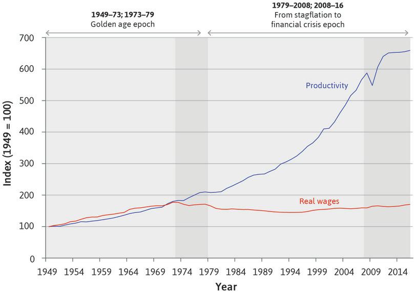
The golden age and its aftermath: Real wages and output per production worker in manufacturing in the US (1949–2016).
Figure 17.17 The golden age and its aftermath: Real wages and output per production worker in manufacturing in the US (1949–2016).
US Bureau of Labor Statistics. Note: ‘production workers’ exclude supervisory employees such as foremen and managers.
The figure shows two dramatically different periods:
- Before 1973: Fair-shares bargaining meant that wages and productivity grew together.
- After 1973: Productivity growth was not shared with workers. For production workers in manufacturing, real wages barely changed in the 40 years after 1973.
By the mid-1990s, the effects of the new supply-side policy regime were becoming clear. The period from this time until the global financial crisis of 2008 was called the great moderation because inflation was low and stable, and unemployment was falling. Although wage growth fell well below productivity growth, policymakers no longer thought of this as a bug; it was a feature of the new regime. The third oil shock that occurred in the 2000s was a good test of the regime. As we saw in Unit 15, it was less disruptive than the two oil shocks in the 1970s.
While the new regime appeared to have the virtue of macroeconomic stability, in countries where the bargaining power of workers had been most curtailed, like the US and the UK, the cost was the dramatic rise in inequality that we saw in Figure 17.2.
In virtually all of the advanced economies, the new supply-side policies redistributed income from wages to profits. In the US (Figure 17.3), the after-tax profit rate gradually increased between the 1970s and 2008. But investment responded only weakly to the profit incentives, so that the rate of growth of the capital stock declined.
Supply-side policy advisors could not recreate the improbable package of high employment, high investment, and growing wages of the golden age. The growth of profits unmatched by investment in new equipment would also help to cause the next crisis.
Exercise 17.3 Workers’ bargaining power
In the light of the Great Depression, most advanced economies adopted policies after the Second World War that strengthened the bargaining power of employees and labour unions. By contrast, after the golden age, the policies chosen weakened workers’ bargaining power.
- Explain the reasons for these contrasting approaches.
- Discuss the possible role of weaker worker bargaining power in the run-up to the global financial crisis.
17.8 Before the financial crisis: Households, banks, and the credit boom
The great moderation masked three changes that would create the environment for the global financial crisis. While to some extent these changes were shared across most advanced economies, actors in the US economy played a pivotal role in the global financial crisis, just as they had during the Great Depression:
- Rising debt: The sum of the debt of the government and of non-financial firms changed relatively little as a proportion of GDP between 1995 and 2008, but the mountainous shape of total debt in the US economy shown in Figure 17.4 was created by growth in household and financial sector debt.
- Increasing house prices: The rise in house prices became more pronounced after 1995.
- Rising inequality: The long-run decline in inequality that began after the Great Depression reversed after 1979 (Figure 17.2). Workers no longer shared in the gains from productivity (Figure 17.17).
How can we make an argument that connects the financial crisis to the great moderation, and to long-run rising debt, house prices, and inequality? We use what we learned in Units 9, 10, 13, and Section 17.4 to help us. We know that during the great moderation, from the mid-1990s to the eve of the financial crisis, the real wages of those with earnings in the bottom 50% hardly grew. Relative to the earnings of the top 50%, they lost out. One way they could improve their consumption possibilities was to take out a home loan. Before the 1980s, financial institutions had been restricted in the kinds of loans they could make and in the interest rates they could charge. Financial deregulation generated aggressive competition for customers, and gave those customers much easier access to credit.
- financial deregulation
- Policies allowing banks and other financial institutions greater freedom in the types of financial assets they can sell, as well as other practices.
- bank bailout
- The government buys an equity stake in a bank or some other intervention to prevent it from failing.
- great recession
- The prolonged recession that followed the global financial crisis of 2008.
The great moderation and the global financial crisis
The great moderation was a period of low volatility in output between the mid-1980s and 2008. It was ended by the global financial crisis, triggered by falling US house prices from 2007 onwards.
- At the onset of the crisis, government and central bank stabilization policies, notably including bank bailouts, avoided a repeat of the Great Depression.
- Nevertheless, there followed a sustained global fall in aggregate output, popularly known as the great recession.
Housing booms and the financial accelerator
When households borrow to buy a house, this is a secured or collateralized loan. As part of the mortgage agreement, the bank can take possession of the house if the borrower does not keep up repayments. Collateral plays an important role in sustaining a house price boom. When the house price goes up—driven, for example, by beliefs that a further price rise will occur—this increases the value of the household’s collateral (see the left-hand diagram in Figure 17.18). Using this higher collateral, households can increase their borrowing, and move up the housing ladder to a better property. This, in turn, pushes up house prices further and sustains the bubble, because the banks extend more credit based on the higher collateral. Increased borrowing, made possible by the rise in the value of the collateral, is spent on goods and services as well as on housing.
- leverage ratio (for banks or households)
- The value of assets divided by the equity stake in those assets.
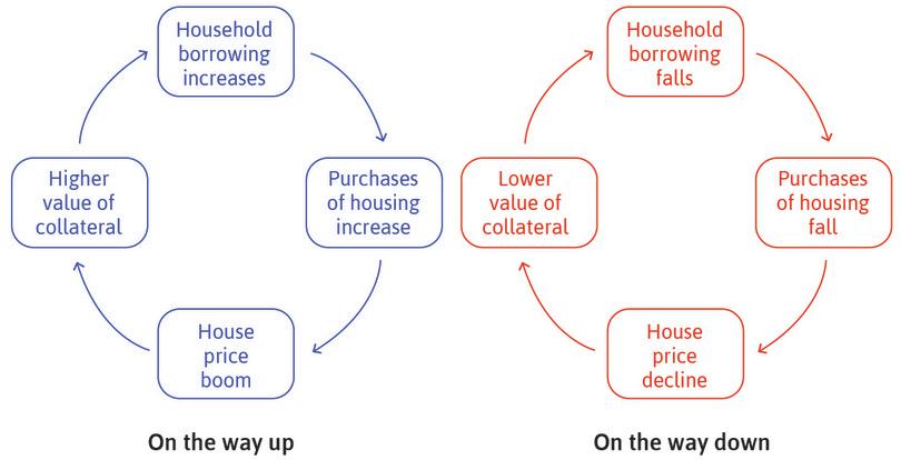
The housing market on the way up and on the way down.
Figure 17.18 The housing market on the way up and on the way down.
Adapted from figure in Hyun Song Shin. 2009. ‘Discussion of ‘The Leverage Cycle’ by John Geanakoplos’.
When house prices are expected to rise, it is attractive to households to increase their borrowing. Suppose a house costs $200,000, and the household makes a down payment of 10% ($20,000). This means it borrows $180,000. Its initial leverage ratio, in this case the value of its assets divided by its equity stake in the house, is 200/20 = 10. Suppose the house price rises by 10% to $220,000. The return to the equity the household has invested in the house is 100% (since the value of the equity stake has risen from $20,000 to $40,000: it has doubled). Households who are convinced that house prices will rise further will want to increase their leverage: that is how they get a high return. The increase in collateral, due to the rise in the price of their house, means they can satisfy their desire to borrow more.
- financial accelerator
- The mechanism through which firms’ and households’ ability to borrow increases when the value of the collateral they have pledged to the lender (often a bank) goes up.
The mechanism through which a rise in the value of collateral leads to an increase in borrowing and spending by households and firms is called the financial accelerator (see Section 14.3 for these details). The left-hand side of Figure 17.18 shows the outcome of the interaction between the bubble in house prices and its transmission through the economy via the financial accelerator during a boom. On the right-hand side, we see what happens when house prices decline. The value of collateral falls and the household’s spending declines, pushing house prices down.
The assets and liabilities of a household can be represented in its balance sheet, and this can be used to explain the interaction of a house price bubble and the financial accelerator. The house is on the asset side of the household’s balance sheet. The mortgage owed to the bank is on the liabilities side. When the market value of the house falls below what is owed on the mortgage, the household has negative net worth. This condition is sometimes referred to as the household being ‘underwater’. Using the example above, if the leverage ratio is 10, a fall in the house price by 10% wipes out the household’s equity. A fall of more than 10% would place the household underwater.
As we saw with households in the Great Depression, if a decline in net worth means that a household is below its target wealth, it responds by cutting what it spends. When a housing bubble is forming, the rise in the value of collateral reinforces the boom by boosting both borrowing and spending; on the way down, the fall in the value of house increases household debt and the household reduces spending. Rising house prices immediately before 2008 were prices that sent the ‘wrong’ message. We know that resources were misallocated, because the US and some countries in Europe were left with thousands of abandoned houses.
Financial deregulation and subprime borrowers
In the boom period when house prices were expected to rise, the riskiness of home loans to the banks making them fell and, as a result, banks extended more loans. The opportunities for poor people to borrow for a home loan expanded as lenders asked for lower deposits, or even no deposit at all. This is shown in Figure 17.19. The financial accelerator mechanism is an example of positive feedback: from higher collateral, to more borrowing, to further increases in house prices.
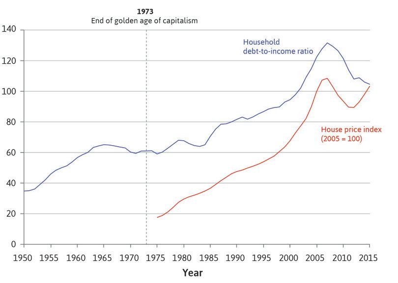
The household debt-to-income ratio and house prices in the US (1950–2015).
Figure 17.19 The household debt-to-income ratio and house prices in the US (1950–2015).
US Federal Reserve. 2016. ‘Financial Accounts of the United States, Historical’. December 10; US Bureau of Economic Analysis; Federal Reserve Bank of St Louis (FRED).
Figure 17.20 shows the contrast between the material wealth of a household in the bottom and top fifth of households, according to their net worth in 2007. Using the definitions introduced in Section 13.3 and used in Section 17.4, the household’s material wealth is equal to the value of its house (which will by definition be equal to the sum of the debt outstanding and the household’s home equity) minus the mortgage debt, plus financial wealth (net of non-housing debt).
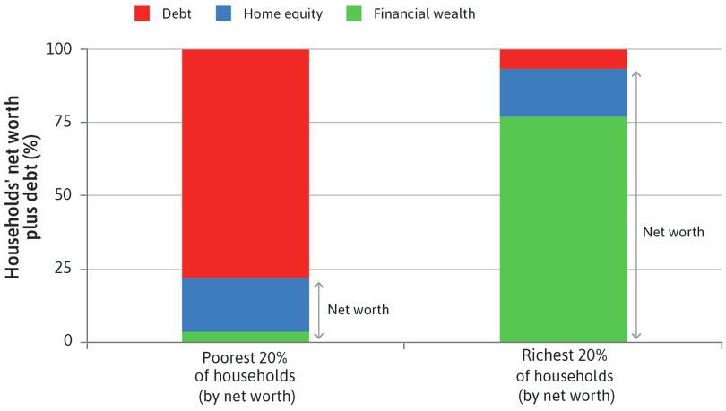
Household wealth and debt in the US: Poorest and richest quintiles by net worth (2007).
Figure 17.20 Household wealth and debt in the US: Poorest and richest quintiles by net worth (2007).
Adapted from Figure 2.1 in Atif Mian and Amir Sufi. 2014. House of Debt: How They (and You) Caused the Great Recession, and How We Can Prevent It from Happening Again. Chicago, Il: The University of Chicago Press.
The left-hand bar is the poorest 20% of households. The right-hand bar is the richest 20%. The data is shown in a way that allows us to compare the assets and liabilities (debt) of the two groups. In each case, the total of debt plus assets is made equal to 100%. This means we cannot compare the absolute amount of wealth or debt held by each group, but the data allows us to see clearly the type of asset (housing or financial) each household type holds, and how much debt each type has relative to the assets it holds. This tells us a lot about how a fall in house prices would affect the spending behaviour of each type.
The left-hand bar represents borrower households. These are poor households, normally only able to borrow when they have housing collateral to use as security. They have little financial wealth, as shown by the size of the green rectangle. These households have much more debt than equity in their houses, and are vulnerable to a fall in house prices.
Rich households have a lot of assets, mainly in the form of financial wealth: bank account and money market deposits, government and corporate bonds, and shares. They also have little debt. These are the saver households of Unit 10.
Financial deregulation and bank leverage
- derivative
- A financial instrument in the form of a contract that can be traded, whose value is based on the performance of underlying assets such as shares, bonds or real estate. See also: collateralized debt obligation.
- collateralized debt obligation (CDO)
- A structured financial instrument (a derivative) consisting of a bond or note backed by a pool of fixed-income assets. The collapse in the value of the instruments of this type that were backed by subprime mortgage loans was a major factor in the financial crisis of 2007–2008.
- mortgage-backed security (MBS)
- A financial asset that uses mortgages as collateral. Investors receive payments derived from the interest and principal of the underlying mortgages. See also: collateral.
- credit ratings agency
- A firm which collects information to calculate the credit-worthiness of individuals or companies, and sells the resulting rating for a fee to interested parties.
In the context of the deregulated financial system, banks increased their borrowing:
- to extend more loans for housing
- to extend more loans for consumer durables like cars and furnishings
- to buy more financial assets based on bundles of home loans
The combination of the great moderation, rising house prices, and the development of new, apparently less risky financial assets such as the derivatives called collateralized debt obligations (CDOs), based on bundles of home loans called mortgage-backed securities (MBSs), made it profitable for banks to become more highly leveraged.
Figure 17.21 shows the leverage of US investment banks and all UK banks.
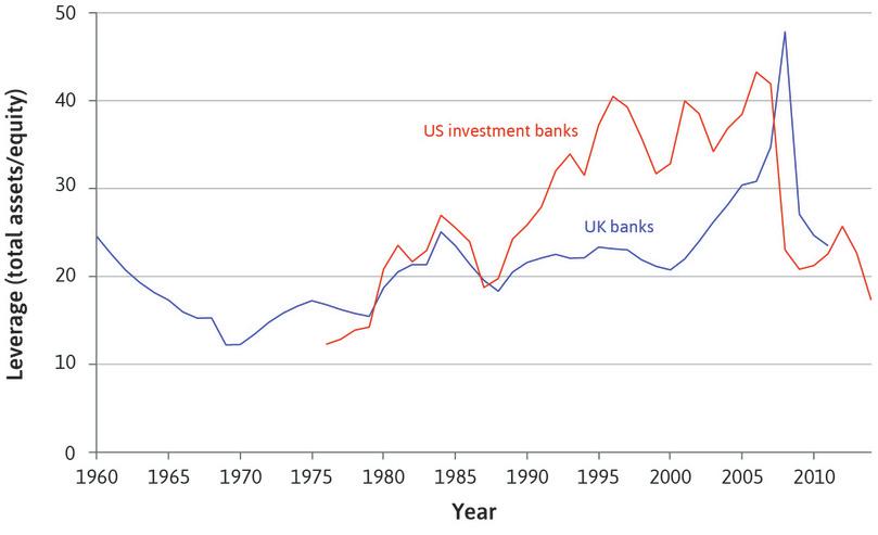
Leverage ratio of banks in the UK and US (1960–2014).
Figure 17.21 Leverage ratio of banks in the UK and US (1960–2014).
US Federal Reserve. 2016. ‘Financial Accounts of the United States, Historical.’ December 10; Bank of England. 2012. Financial Stability Report, Issue 31.
In the US, the leverage ratio of investment banks was between 12 and 14 in the late 1970s, rising to more than 30 in the early 1990s. It hit 40 in 1996 and peaked at 43 just before the financial crisis. By contrast, the leverage of the median UK bank remained at the level of around 20 until 2000. Leverage then increased very rapidly to a peak of 48 in 2007. In the 2000s, British and European global banks, including firms called shadow banks, increased borrowing to buy CDOs and other financial assets that originated in the US housing market.
Leverage increased because of financial deregulation and the business model of banks. But why were savers prepared to continue lending to the increasingly leveraged financial system and, indirectly, to the highly leveraged household sector?
Firms called credit ratings agencies (the big three are Fitch Ratings, Moody’s and Standard & Poor’s) assess the risk of financial products, and part of their role is to provide evidence to reassure lenders that their investments are safe. After almost 20 years of the great moderation, economic crises seemed like a historical idea, and so these companies gave the highest ratings (meaning the lowest risk) to many of the assets created from subprime mortgages.
- subprime mortgage
- A residential mortgage issued to a high-risk borrower, for example, a borrower with a history of bankruptcy and delayed repayments. See also: subprime borrower.
The subprime housing crisis of 2007
The interrelated growth of the indebtedness of poor households in the US and global banks meant that when homeowners began to default on their repayments in 2006, the effects could not be contained within the local or even the national economy. The crisis caused by the problems of subprime mortgage borrowers in the US spread to other countries. Financial markets were frightened on 9 August 2007 when French bank BNP Paribas halted withdrawals from three investment funds because it could not ‘fairly’ value financial products based on US mortgage-based securities—it simply did not know how much they were worth.
The recession that swept across the world in 2008–09 was the worst contraction of the global economy since the Great Depression. Unlike the bushfires in southeastern Australia in 2009, the financial crisis took the world by surprise. The world’s economic policymakers were unprepared. They discovered belatedly that a long period of calm in financial markets could make a crisis more likely.
This was an argument that Hyman Minsky, the economist, had made long before the great moderation. Minsky developed these ideas while a professor of economics at the University of California, Berkeley, and so he may even have been thinking of fires. In northern Mexico, the fire management authorities allow small fires to burn, and as a result dry undergrowth does not accumulate. Major fires are more frequent across the US border in California, where small fires are quickly extinguished.
In 1982, Minsky wrote Can ‘It’ Happen Again? about the way in which tranquil conditions lead firms to choose riskier methods of financing their investment.4 His warning went unheeded. Instead of producing increased vigilance, the calm conditions of the great moderation bred complacency among regulators and economists. It was the increasingly risky behaviour of banks, as Minsky had predicted, that created the conditions for the crisis.
Great economists Hyman Minsky
Hyman Minsky (1919–1996) was an American economist who developed a financial theory of the business cycle. His ideas have attracted renewed attention among both academics and banking and finance professionals since the global economic crisis of 2008.
Minsky argued that macroeconomic fluctuations could not be properly understood without taking account of the manner in which business investment is financed. At a time when most economists viewed firms as the location of a production function, Minsky focused instead on the assets and liabilities on the firm’s balance sheet. The assets, including plant and equipment, but also less tangible assets such as patents, copyrights, and trademarks, are expected to generate a stream of revenues stretching far into the future. The liabilities include the firm’s obligations to its creditors, and imply a stream of payments due at various points in time.
- hedge finance
- Financing used by firms to fulfil contractual payment obligations using cashflow. Term coined by Hyman Minsky in his Financial Instability Hypothesis. See also: speculative finance.
- speculative finance
- A strategy used by firms to meet payment commitments on liabilities using cash flow, although the firm cannot repay the principal in this way. Firms in this position need to ‘roll over’ their liabilities, usually by issuing new debt to meet commitments on maturing debt. Term coined by Hyman Minsky in his Financial Instability Hypothesis. See also: hedge finance.
New investment by the firm expands its capacity to produce goods and services, and thus alters its expected stream of revenues. If it is financed by debt, it also changes the firm’s financial obligations at future dates. In deciding how to finance its investment, the firm faces a choice:
- Issue long-term debt: It anticipates that revenues would be sufficient to cover obligations at all points in time.
- Issue short-term debt: This debt needs to be repaid before the anticipated revenues are available. It creates the need for further borrowing to repay debt at the end of this term.
In general, long-term borrowing is more expensive, since lenders demand a higher interest rate. But short-term borrowing is risky, because the firm may be unable to refinance debt as it comes due. Even if it can refinance, it may be forced to borrow at high rates if credit availability is constrained.
Firms that chose the safer but more expensive option, matching revenues and debt obligations, were said by Minsky to be engaged in hedge finance. Those that took the cheaper but more risky option, borrowing short-term to finance long-term investments, were engaging in speculative finance.
A key component of Minsky’s theory concerned the manner in which the distribution of financial practices in the economy changed over time. As long as financial market conditions remained relatively tranquil, so that rolling over short-term debt was easy, firms with the most aggressive financial practices would prosper at the expense of those that were the most prudent. Not only would the most aggressive firms grow faster, they would also attract imitators, and the distribution of financial practices in the economy would become increasingly speculative. There would be a rise in the demand for refinancing short-term debt, and hence an increase in financial fragility: a severe financial market disruption, with a contraction in credit or a spike in short-term interest rates, would become increasingly likely.
In Minsky’s view, this process leads inevitably to a crisis because, as long as a crisis is averted, the most aggressive financial practices proliferate and financial fragility continues to rise. When a crisis finally occurs, the most aggressive firms will suffer disproportionately and the prudent firms will prosper. The sharp shift in the aggregate distribution of financial practices lowers fragility and sets the stage for the process to begin again. In Minsky’s words:
Stability—even of an expansion—is destabilizing in that more adventurous financing of investment pays off to the leaders, and others follow. (John Maynard Keynes, 1975)
In other words, a period like the great moderation sows the seeds of the next financial crisis.
In 2007, Charles Prince, chief executive of Citigroup, explained to the Financial Times the difficulty of resisting ‘adventurous financing’ during booms. ‘As long as the music is playing, you’ve got to get up and dance,’ he said in July, as the global economy hurtled towards a crisis deeper than anything seen since the Great Depression, ‘We’re still dancing’.
Exercise 17.4 Household wealth as a balance sheet
- Show the information in Figure 17.20 in the form of a balance sheet, for one household from the lowest and one from the highest net worth quintile (use the balance sheets in Figures 10.16 and 10.17 as a guide). Assume that the sum of assets and liabilities is $200,000 for the poorer household and $600,000 for the richer household, both households have some savings, and that assets do not depreciate.
Think about the proportions of debt held by these households that might consist of mortgage debt. Now consider the relative effects on the households of a fall in house prices.
- Define negative equity as a situation where the market value of a house is less than the debt secured on it. In your example balance sheet for the poorer family, calculate the fall in house prices that would push this household into negative equity.
- If house prices fell by just enough to push the household into negative equity, would this household be insolvent? Explain.
Question 17.8 Choose the correct answer(s)
Figure 17.19 shows the household debt-to-income ratio and the house prices in the US between 1950 and 2014. Based on this information, which of the following statements is correct?
- It is not the real value but the ratio in proportion to household income that has more than doubled in the 35 years.
- There exists a positive feedback in both directions (the financial accelerator). Thus not only do higher house prices encourage higher debt via rising collateral values, but higher debt leads to higher prices through increased demand.
- A household debt-to-income ratio of over 100 does not necessarily mean that the household is bankrupt. In a low interest rate environment such a high debt level can still be maintained. A household is bankrupt if its debt is higher than its assets, not its income.
- Some of the rise in household debt in the US was lent as mortgages to households who could not really afford to repay.
Question 17.9 Choose the correct answer(s)
Figure 17.21 is the graph of leverage of banks in the UK and the US between 1960 and 2014.
The leverage ratio is defined as the ratio of the banks’ total assets to their equity. Which of the following statements are correct?
- 2.5% equity means total assets are equal to 40 times the value of equity.
- Doubling of the leverage does not imply that the value of assets has doubled. The leverage could double even if the asset value is constant, if the amount of equity is halved.
- If assets fall by 4% then they lose one twenty-fifth of their value, which is exactly the value of the equity. This would imply a net worth of zero, so the bank would be just insolvent.
- UK banks increased their borrowing not to lend to UK house buyers directly, but to buy CDOs and other financial assets which originated in the US housing market.
17.9 Modelling housing bubbles
In Unit 11 (Section 11.8), we introduced the concepts of stable and unstable equilibria. Here we develop those concepts further. We will show that a market like the housing market can have a stable equilibrium at a low price and another stable equilibrium at a high price level. In between is an unstable equilibrium. This is represented by an S-shaped price dynamics curve (PDC).
Figure 17.22 reproduces diagrams from Figures 11.18 and 11.19. The left hand panel shows what happens at an unstable equilibrium. Beginning at the price P₀, an increase in the price leads away from equilibrium because it is interpreted as a sign that the price will rise further, which drives up demand for houses as people demand more of the asset they believe will increase in value. If at the price P₀ something were to occur that lowered the price, a similar process would take the price even lower, as people would take that to be a signal that houses are falling in value, and so would be less likely to buy.
The right-hand panel shows how a stable equilibrium is one in which initial price changes are dampened rather than exaggerated as a result of what is called negative feedback. Here a rise in price leads to a fall in demand for houses, which depresses the price. Eventually the price returns to the initial level. This is a stable equilibrium.
- negative feedback (process)
- A process whereby some initial change sets in motion a process that dampens the initial change. See also: positive feedback (process).
- positive feedback (process)
- A process whereby some initial change sets in motion a process that magnifies the initial change. See also: negative feedback (process).
The process that leads a market to adjust to a small shock by returning to its pre-existing equilibrium is called a negative feedback process because the initial price change causes further price changes (feedbacks) that are in the opposite direction (negative) of the initial change. A positive feedback process is one in which some initial change leads to further changes in the same direction (positive).
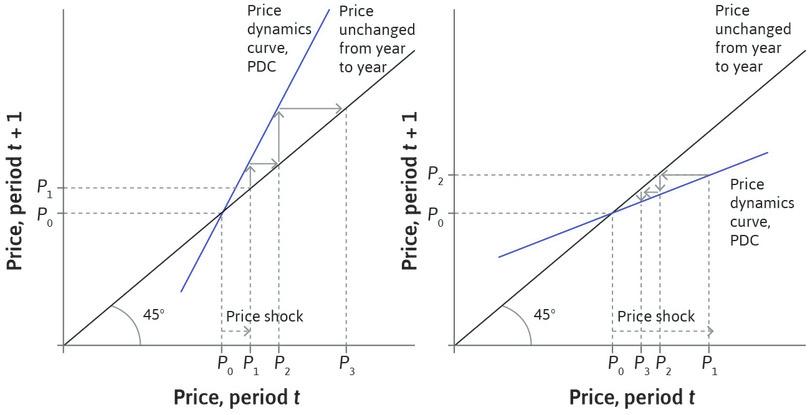
Unstable and stable equilibria in the housing market.
Figure 17.22 Unstable and stable equilibria in the housing market.
In order to see how a market could have two equilibria and how movement from one to the other could represent a price bubble or a price crash, we can combine the stable and unstable equilibria in the two panels of Figure 17.22 into the S-shaped figure shown in Figure 17.23. Notice that at A the PDC has a slope that is steeper than 45 degrees (like the left panel in Figure 17.22). So point A is an unstable equilibrium and the price will not remain here if it is disturbed by either a price rise or fall no matter how small: positive feedbacks will lead the price away from the equilibrium. There will be a house price bubble if the price increases at A, and a crash if the price decreases.
Notice that at points C and B the PDC is flatter that the 45-degree line, so for these points the right panel of Figure 17.22 explains what will happen if the market is at either one of these points and something shifts the price up or down. Because of negative feedback, the initial shock will be dampened and the price will return to the equilibrium value.
Point A is called a tipping point. For a price above A, prices increase continuously until point B; for a price below A, prices decrease continuously until point C. The direction of the change in price switches from rising to falling at the tipping point A.
Tipping point
An unstable equilibrium at the boundary between two regions characterized by distinct movements in some variable. If the variable takes a value on one side of the tipping point, the variable moves in one direction; on the other, it moves in the other direction. A ridge dividing two valleys is a tipping point; for example, water falling on one side runs away from the ridge in one direction towards an inland lake while water falling on the other side (even very close to the ridge) flows in the other direction towards the sea. In the case of the housing bubble, beyond a certain price (the tipping point price), prices will increase creating a bubble and below that price they fall (a bust).
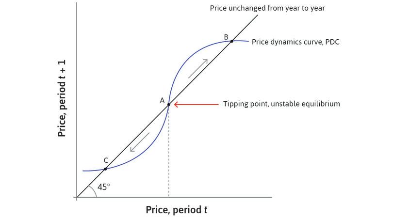
Unstable and stable equilibria in the housing market: The S-shaped PDC.
Figure 17.23 Unstable and stable equilibria in the housing market: The S-shaped PDC.
Remember that at B, house prices are high, but stable. They will remain unchanged at the high level from year to year. Even if there are blips up or down, we know that the price will return to its level at B.
But now suppose that at the high price (point B) some people ‘get cold feet’. They think prices are far too high given the fundamentals of house affordability (the demand side) and the supply of houses. ‘These high prices can never last,’ they say to themselves. They begin to think that house prices will fall: ‘It’s time to sell so that when prices fall, I can get a better house for the same money.’ Owners with a mortgage start to worry that lower house prices could leave them with negative equity in their house, that is, a situation in which the market value of the house is less than the mortgage they owe to the bank.
These people will believe that house prices are going to be lower next period than shown by B. This is represented in Figure 17.24 by a downward shift of the S-shaped price dynamics curve to the darker blue one. As more people come round to the view that prices will fall and sell their houses, the S-shaped curve shifts down and prices fall along the broken arrow from B to Z.
Once sentiment in the housing market has shifted sufficiently that the S-shaped curve (now dark blue) is below the 45-degree line, there is no tipping point left. The market collapses to K. This model helps to explain the fear that a bubble in the housing market can be followed by a devastating crash. Note that the financial accelerator is part of the reason why these collapses can be so large and why the new equilibrium can be so far below the old equilibrium.
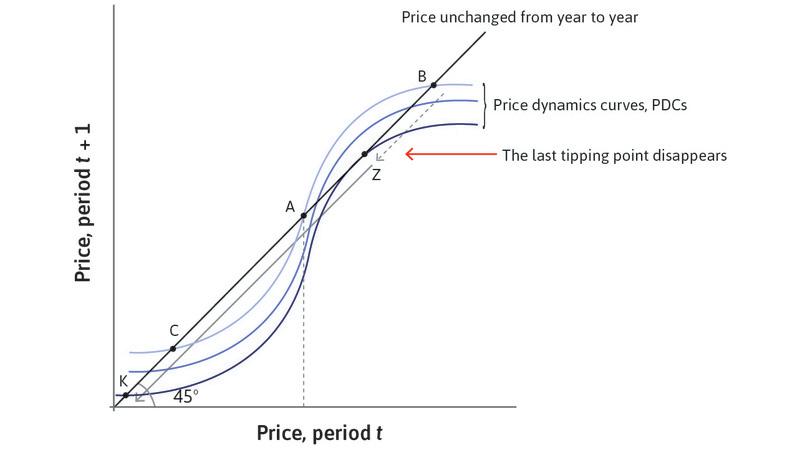
A tipping point in the housing market.
Figure 17.24 A tipping point in the housing market.
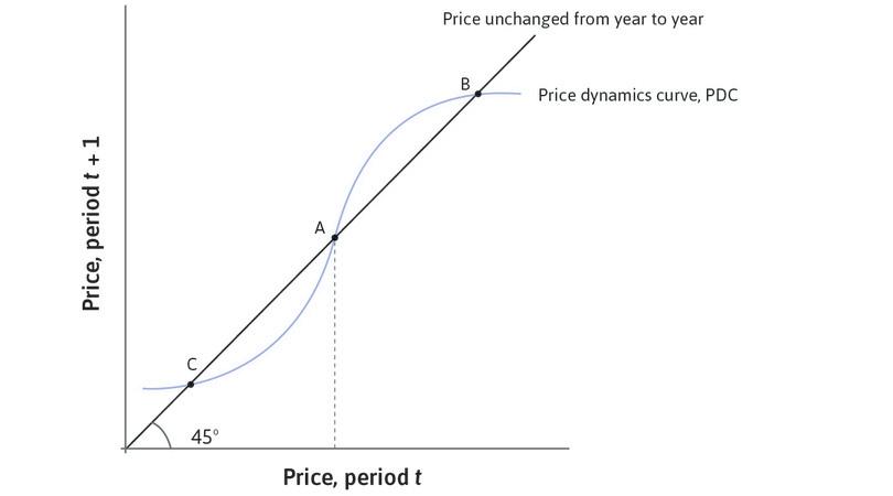
An equilibrium at B
At Point B, house prices are high, but stable.
Figure 17.24a At Point B, house prices are high, but stable.
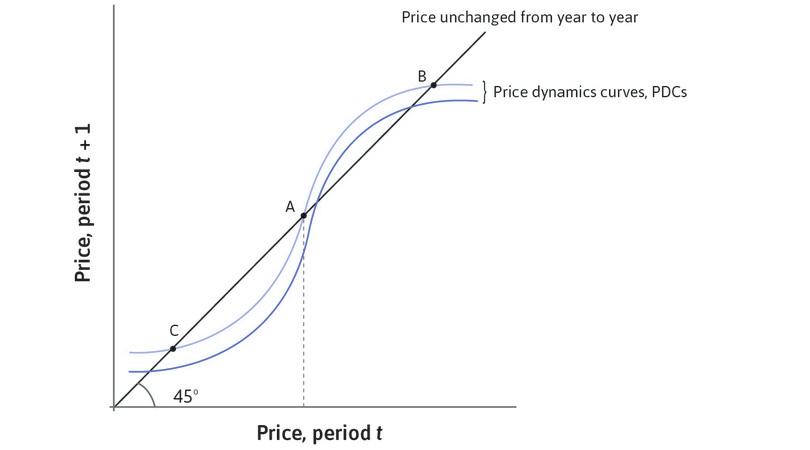
Some owners get ‘cold feet’
Suppose some people start to believe that prices are too high and sell their houses. This is shown by a downward shift of the S-shaped price dynamics curve to the darker blue one.
Figure 17.24b Suppose some people start to believe that prices are too high and sell their houses. This is shown by a downward shift of the S-shaped price dynamics curve to the darker blue one.
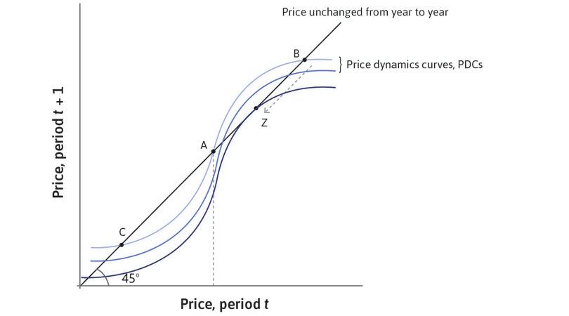
A change in sentiment
As more people come round to the view that prices will fall and also sell, the S-shaped curve shifts down and prices fall along the broken arrow from B to Z.
Figure 17.24c As more people come round to the view that prices will fall and also sell, the S-shaped curve shifts down and prices fall along the broken arrow from B to Z.
Prices collapse
The sentiment in the housing market has shifted so much that there is no tipping point left. The market collapses to K.
Figure 17.24d The sentiment in the housing market has shifted so much that there is no tipping point left. The market collapses to K.
Exercise 17.5 Differences between equilibrium and stability
Explain in your own words, giving examples, the difference between the terms equilibrium and stability.
Question 17.10 Choose the correct answer(s)
Figure 17.24 shows some S-shaped price dynamics curves for the housing market.
Based on the figure, which of the following statements is true?
- At these points, next period’s price will be a movement towards a stable equilibrium, in the opposite direction from the initial shock.
- Point Z is an unstable equilibrium, but point K is a stable equilibrium.
- A positive feedback process could result in housing prices decreasing, for example, on the pale blue PDC, a negative shock at point A would cause housing prices to decrease until the intersection between the pale blue PDC and the 45-degree line.
- Optimism would result in higher prices for both of the stable equilibria (the opposite of what the figure shows).
17.10 The financial crisis and the great recession
Rising house prices in the US in the 2000s were driven by the behaviour of lenders, encouraged by government policy, to extend loans to poorer households. They were able to fund these subprime loans by packaging them into financial derivatives, which banks and financial institutions across the world were eager to buy. Rising house prices created the belief that prices would continue to rise, which shifted the demand curve for housing further to the right by providing households with access to loans based on housing collateral.
Follow the steps in the analysis in Figure 17.25 to see the housing price cycle on the way down from its peak in mid-2006. It illustrates how a small initial fall in prices led to a further collapse in demand as people started to believe that house prices would fall further. This change in beliefs resulted in the downward shift in the PDC in Figure 17.24, creating a new lower equilibrium value for house prices.
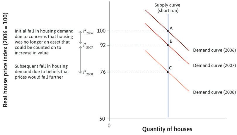
The financial crisis: The US housing price collapse.
Figure 17.25 The financial crisis: The US housing price collapse.
Bank for International Settlements. 2015. ‘Residential Property Price Statistics’. Updated November 20, and other national sources.
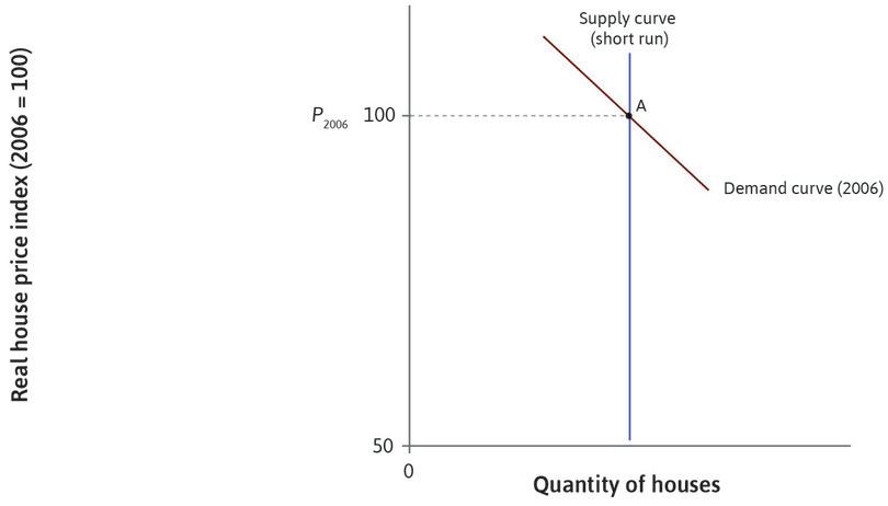
The US economy (2006)
The housing market in the US economy in 2006 is shown at point A.
Figure 17.25a The housing market in the US economy in 2006 is shown at point A.
Bank for International Settlements. 2015. ‘Residential Property Price Statistics.’ Updated November 20, and other national sources
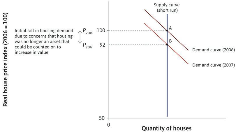
House prices fall (2007)
House prices began to decline in 2007 as demand shifted downwards from A to B, pushing the house price index down to 92 from its peak of 100.
Figure 17.25b House prices began to decline in 2007 as demand shifted downwards from A to B, pushing the house price index down to 92 from its peak of 100.
Bank for International Settlements. 2015. ‘Residential Property Price Statistics.’ Updated November 20, and other national sources
A positive feedback process
Once prices were falling, the belief that prices would fall further became widespread. This led to further declines in demand, all the way down to C. The house price index fell to a level of 76 in 2008.
Figure 17.25c Once prices were falling, the belief that prices would fall further became widespread. This led to further declines in demand, all the way down to C. The house price index fell to a level of 76 in 2008.
Bank for International Settlements. 2015. ‘Residential Property Price Statistics.’ Updated November 20, and other national sources
In Figure 17.26 you can see the contribution of the components of GDP to growth in the 18 months before the crisis in the US economy, then in the five quarters of recession from the start of 2008, followed by the recovery phase to the end of 2010. The fall in residential investment (the red bar) was the most important feature of the onset phase. At that stage, it was the only drag on growth. This was the consequence of the fall in house prices that began in late 2006. During the recession, a further fall in housing investment was compounded by a fall in non-residential investment and consumption.
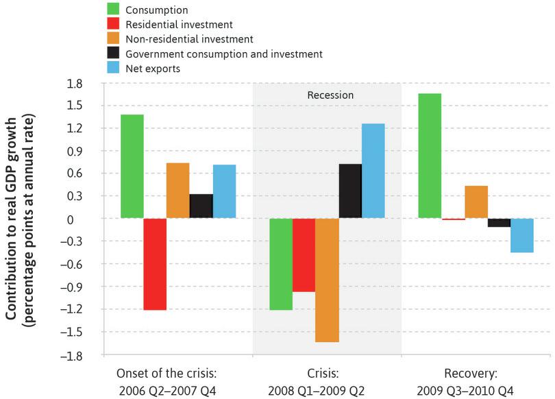
Aggregate demand and the financial crisis in the US (2006 Q2–2010 Q4).
Figure 17.26 Aggregate demand and the financial crisis in the US (2006 Q2–2010 Q4).
Just as in the Great Depression, the fall in consumption was not simply due to the multiplier process. Households stopped buying new houses, but also cut spending on consumer durables. The financial accelerator mechanism helps to explain the transmission of falling house prices through the fall in the value of collateral to aggregate demand. Cutbacks in spending on new housing and on consumer durables were concentrated among the poorer households who had taken out subprime mortgages. The timing of the collapse of demand is consistent with the central role played by housing and debt in the financial crisis. There was also a fall in investment. Orders for new equipment were cancelled and factories closed. Workers were laid off and job creation slumped.
We can link the pattern of aggregate demand in Figure 17.26 to the decisions of households by using a diagram similar to the one we developed for the Great Depression. This is Figure 17.27. These two figures are different ways of looking at the same developments: Figure 17.27 is an individual household’s view of the unfolding crisis, while Figure 17.26 is the same process from the perspective of the whole economy.
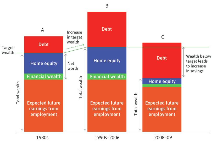
The financial crisis: Housing boom, household debt, and house price crash.
Figure 17.27 The financial crisis: Housing boom, household debt, and house price crash.
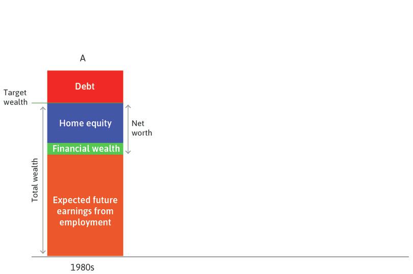
The great moderation (1980s)
Column A shows the situation in the 1980s.
Figure 17.27a Column A shows the situation in the 1980s.
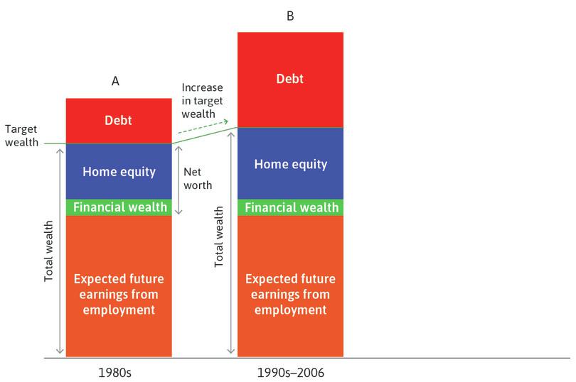
Rising house prices (1990s–2006)
Through the 1990s and especially in the early 2000s, rising house prices increased total wealth, so households increased consumption by increasing debt.
Figure 17.27b Through the 1990s and especially in the early 2000s, rising house prices increased total wealth, so households increased consumption by increasing debt.
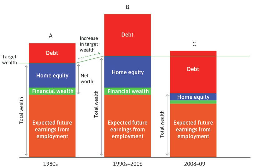
Falling house prices (2006–2009)
Rising unemployment led to a downward re-evaluation of expected future earnings from employment. Household net worth shrank.
Figure 17.27c Rising unemployment led to a downward re-evaluation of expected future earnings from employment. Household net worth shrank.
Wealth is below target
The fall in house and asset prices, combined with lower expected earnings, reduced wealth below target. Households cut consumption and increased savings.
Figure 17.27d The fall in house and asset prices, combined with lower expected earnings, reduced wealth below target. Households cut consumption and increased savings.
Column A in Figure 17.27 shows the situation in the 1980s. The 1990s to mid-2000s, as we saw, was a period of rapidly rising house prices. Column B shows the outcome by 2006. In the figure, the house price is the sum of the blue box for home equity, and the red box for debt (the mortgage). The increase in house prices increased home equity and pushed up households’ assessment of their wealth, which was inflated by the expectation that house prices would continue to rise. One effect was that they uprated their target wealth. But target wealth did not grow as much as perceived wealth, so they also borrowed more in order to consume more. This meant that home equity grew, but so did debt. The higher level of household debt is shown by the larger debt rectangle in column B.
From 2006, house prices in the US began to fall. The household’s viewpoint in 2008 and 2009 is shown in column C. Rising unemployment led to a downward re-evaluation of expected future earnings from employment. Household net worth shrank, as we can see in column C. Note that the size of the debt rectangle has not changed between columns B and C. The combined effect of the fall in house and asset prices, the increased debt acquired in the boom years, and lower expected earnings, had the effect of reducing wealth below target. As a result, households cut consumption and increased savings. This is shown in column C by the double-headed arrow labelled ‘Wealth below target leads to increase in savings’.
The household shown in Figure 17.27 still has positive net worth following the fall in house and asset prices in the crisis. This is shown by the sum of the red, blue, and green rectangles in column C. But the behaviour of households whose net worth became negative following the fall in house prices was an important feature of the great recession that followed the financial crisis in the US. To show this in a diagram like Figure 17.27, the debt rectangle would slide down into the box labelled ‘expected earnings from employment’, wiping out the blue, green, and orange rectangles, reducing total wealth, and increasing the gap between expected and target wealth. It is easy to see how households in the bottom quintile shown in Figure 17.20 went underwater in 2008 and 2009. In the US in 2011, 23% of properties with a mortgage were worth less than that mortgage. Households in this position would have cut consumption as they paid down their debt to restore their financial position.
Exercise 17.6 The crisis and the multiplier
- Show the features of the 2008 crisis in the multiplier diagram, using Figure 14.6 for the Great Depression as a model. Use the concepts of the consumption function, a house price bubble, the financial accelerator, and positive feedback in your answer.
- How can you represent the role played by the higher marginal propensity to consume of households in the bottom quintile in your analysis? Refer to Figure 17.20 and assume the economy is closed.
Question 17.11 Choose the correct answer(s)
Figure 17.26 depicts the US aggregate demand between 2006 Q2 and 2010 Q4.
Based on this information, which of the following statements is correct?
- It cannot be stated that the fall in residential investment was the sole cause of the crisis. This fall itself was a consequence of the fall in house prices that began in 2006.
- Non-residential investment was the single greatest contributor, as indicated by the orange column in the crisis period.
- Government consumption and investment were increased to counter economic contraction during the recession, but they have since been cut back.
- In the recovery period, household consumption grew but there was still no growth in residential investment.
17.11 The role of banks in the crisis
House prices and bank solvency
The financial crisis was a banking crisis—and it was global, as BNP Paribas demonstrated in August 2007 when it would not pay out to bondholders in one of its investment funds. The banks were in trouble because they had become highly leveraged and were vulnerable to a fall in the value of the financial assets that they had accumulated on their balance sheets (refer back to Figure 17.21 for the leverage of US and UK banks). The values of the financial assets were in turn based on house prices.
With a ratio of net worth to assets of 4%, as in the example of the bank in Figure 11.14, a fall in the value of its assets of an amount greater than this will render a bank insolvent. House prices fell much more than 4% in many countries in the recent financial crisis. In fact, the peak-to-trough fall in house price indices for Ireland, Spain, and the US were 50.3%, 31.6%, and 34.6% respectively. This created a problem of solvency for the banks. Just as with the underwater households, banks were in danger of their net worth being wiped out. It is relatively easy for a household to calculate whether this has happened, but not for a bank.
Unlike a house, obscure financial assets on (or often designed to be kept off) a bank’s balance sheet, with acronyms like CDO, CDS, CLO, and even CDO², were hard to value. This made it difficult to judge which banks were in trouble.
Bank liquidity and the credit crunch
- liquidity risk
- The risk that an asset cannot be exchanged for cash rapidly enough to prevent a financial loss.
Doubts about the solvency of banks created another problem in the financial system—the problem of liquidity risk, which we introduced in Unit 10. A characteristic feature of banking is the mismatch between short-term liabilities, which it owes to depositors, and long-term assets, which are loans owed to the bank. Consequently, banks rely on the money market, where banks borrow from and lend to each other on a short-term basis, to fund themselves when they need short-term liquidity. But the operation of the money market relies on borrowers and lenders having trust in the solvency of those with whom they trade. The expected profit on a loan is the interest rate multiplied by the probability that the borrower will not default:
Therefore, as people feared that those to whom they were lending were more likely to default, they would only lend at a high interest rate. In many cases, banks or others operating in the money markets simply refused to lend at all. Newspapers called it the ‘credit crunch’.
In Unit 10, we learnt that the interest rate in the money market is tied tightly to the policy interest rate set by the central bank. This relationship broke down in the credit crunch. Borrowing on the interbank market became much more expensive and hampered the ability of central banks to stabilize the economy. Even when the central banks reduced the interest rate close to the zero lower bound, the fear that banks would default kept money market rates high. This led to high mortgage lending rates: high money-market interest rates raised a bank’s funding costs, as discussed in Unit 10.
Fire sales: A positive feedback process
- fire sale
- The sale of something at a very low price because of the seller’s urgent need for money.
The forced sale of assets, known informally as a fire sale, is a positive feedback process. In the financial crisis, the fire sale is an external effect for both the housing market and the markets for financial assets, and both affected the solvency of banks.
In the housing case, it is easy to visualize. Think of a household that is underwater and cannot repay a housing loan. Its debt exceeds the market value of the house. The household is under pressure to sell quickly in order to pay off as much of the mortgage as they can, to avoid continuing interest payments. If the housing market is undergoing a crash, then they may have to accept a drastically reduced price for the house (which may still be better for them than continuing to pay interest on the whole mortgage). This is a market failure because the fire sale has an external effect, conferring a cost (a fall in price) on other owners of the same type of asset.
In the financial crisis, banks as well as households faced massive losses in the value of their financial assets and were under pressure to sell them at reduced prices in order to repay debts (for example, to depositors who wanted their deposits back). Since many banks were desperately trying to sell at the same time, these asset prices plunged. This in turn further threatened the solvency of banks and other financial institutions as part of the positive feedback loop.
Governments rescue banks
Across the advanced economies, banks failed and were rescued by governments. To find out more about how they did this, and for more background on how the financial system failed during the crisis, we suggest reading The Baseline Scenario.
In Unit 10 we highlighted the fact that banks do not bear all the costs of bankruptcy. The bank owners know that others (taxpayers or other banks) will bear some of the costs of the banks’ risk-taking activity. So the banks take more risks than they would take if they bore all the costs of their actions. Excess risk-taking by banks is a negative external effect leading to a market failure. And it arises because of the principal-agent problem between the government (the principal) and the agent (the bank). The government is the principal because it has a direct interest in (and is held responsible for) maintaining a healthy economy, and will bear the cost of bank bailout as a consequence of excessive risk-taking by banks. Governments cannot write a complete set of rules that would align the interests of the banks with those of the government or the taxpayer.
Banks are rescued because the failure of a bank is different from the failure of a typical firm or household in a capitalist economy. Banks play a central role in the payments system of the economy and in providing loans to households and to firms. Chains of assets and liabilities link banks, and those chains had extended across the world in the years before the crisis.
The interconnectedness of banks was vividly illustrated in the credit crunch, where liquidity dried up in the money markets because each bank doubted the solvency of other banks. The event associated most closely with the financial crisis, the bankruptcy of US investment bank Lehman Brothers on 15 September 2008, showed how interconnected banks were (and are). This was not the beginning of the crisis—we have seen that the contraction of aggregate demand in the US began with the troubles in the housing market—but it signalled its escalation at the national and global level.
Thus the banking system, like an electricity grid, is a network. The failure of one of the elements in this connected network—whether a household or another bank—creates pressure on every other element. Just as happens in an electricity grid, the process in a banking system may create a cascade of subsequent failures, as occurred between 2006 and 2008.
In our ‘Economist in action’ video, Joseph Stiglitz, one of the few economists who warned repeatedly about the risks inherent in the financial system in the lead-up to the financial crisis, explains the combination of incentives, external effects, and positive feedback processes that led to this cascade of financial failure.

Exercise 17.7 How conventional wisdom on financial markets contributed to the global financial crisis
In the ‘Economist in action’ video of Joseph Stiglitz he explains that the financial crisis was a market failure. Watch it, and consider these questions:
- What assumptions were made about financial markets before the crisis, and which assumption was particularly problematic?
- How did incentives given to banks play a role in the recent financial crisis?
Exercise 17.8 Behaviour in the financial crisis
‘The Crisis of Credit Visualized’ is an animated explanation of the behaviour of households and banks in the financial crisis available on YouTube.
- Use the models discussed in this unit to explain the story told in the video.
- Are there parts of the video that you cannot explain using the models and concepts from this unit?

Question 17.12 Choose the correct answer(s)
Which of the following statements are correct regarding fire sales in the housing market?
- This is the definition of an ‘underwater’ household.
- A fire sale is when an asset is sold in a hurry at a low price in order to avoid bankruptcy or illiquidity. In a normal housing market, a household that cannot repay its mortgage (perhaps because of job loss) might be able to sell at a normal price.
- An externality is an unintended effect on parties not involved in the transaction. The possibility of buyers benefitting from cheaper prices is not an externality because they are parties to the transaction.
- This is a negative externality because owners of similar assets are not parties to this particular transaction.
17.12 The economy as teacher
Economists learned about the importance of aggregate demand from the Great Depression, but it gave them an undue confidence that a combination of fiscal and monetary policy would virtually eliminate unemployment in the long run. In Section 17.6, we saw the limits to this policy when the golden age broke down, with intensified conflict between workers and employers reflected in rising inflation.
The dominance of the prevailing Keynesian aggregate demand-oriented view helps explain most economists’ failure to diagnose the supply-side nature of the first oil shock in 1973. Figure 17.28 illustrates this policy mistake for the US. The doubling of the oil price (in real terms) is indicated by the increase in the index from 5 to 10 in the chart in 1973. From Unit 15 and this unit, we know that when the national economic pie is reduced by a commodity price shock, this will intensify the conflict of interest over its division, and so inflation increased to more than 10% in 1974. Yet policymakers were focused on the effect of the oil price shock in reducing aggregate demand and raising unemployment. They responded by loosening monetary policy (look at the falling nominal and real interest rates). Fiscal policy was not tightened.
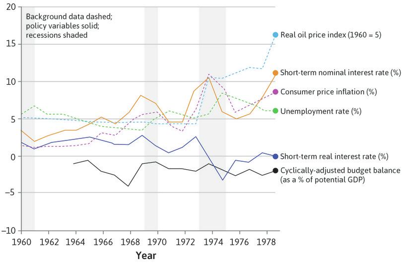
Policy choices during the end of the golden age: The US (1960–79).
Figure 17.28 Policy choices during the end of the golden age: The US (1960–79).
Federal Reserve Bank of St Louis (FRED); Congressional Budget Office; US Bureau of Labor Statistics.
A different response followed the second oil shock in 1979. The focus was on the need to reduce inflation and to restore expected profits. Instead of attempting to support aggregate demand, policymakers paid attention to the upward pressure on inflation created by the oil shock. Monetary and fiscal policy were directed toward the control of inflation as advocated by Milton Friedman a decade earlier; policy was tightened and governments were prepared to allow unemployment to rise in order to reduce inflation.
Expressed in terms of the labour market model, policymakers now recognized that the oil shock raised the inflation-stabilizing unemployment rate, which led them to implement supply-side policies to weaken trade unions (to shift the wage-setting curve down) and to increase competition in monopolized industries such as telecommunications (to shift the price-setting curve up). These policies were closely associated with Prime Minister Margaret Thatcher in the UK and President Ronald Reagan in the US.
By extending deregulation from labour and product markets to the financial system, policymakers of the post-1979 epoch created the conditions in which financial practices that led to the global financial crisis could proliferate. Hyman Minsky had warned as early as 1982 how this could occur in tranquil macroeconomic circumstances.
Some had echoed Minsky’s thinking well before the crisis. For example, in September 2000, Sir Andrew Crockett, general manager at the Bank for International Settlements, told banking supervisors:
The received wisdom is that risk increases in recessions and falls in booms. In contrast, it may be more helpful to think of risk as increasing during upswings, as financial imbalances build up, and materializing in recessions.5
In the table in Figure 17.29 we summarize the lessons for economists from each epoch.
| Epoch | Dates | Prior conventional wisdom | Economic outcomes | What economists learned | Primary author |
|---|---|---|---|---|---|
| 1920s and the Great Depression | 1921–1941 | Markets are self-correcting, efficient, and ensure the full use of resources. | Collapse of aggregate demand, high and persistent unemployment. | Instability is an intrinsic feature of the aggregate economy and aggregate demand can be stabilized by government policy. | Keynes |
| Golden age of capitalism and its demise | 1945–1979 | Government policy can implement an employment target by picking a point on the Phillips curve. | Late-60s decline in profits, investment, and productivity growth. Stable Phillips curve trade-off disappears. |
With given institutions, the need to maintain profits, investment, and productivity growth can limit the ability of a government to implement sustainable low unemployment using aggregate demand policies. | Friedman |
| From stagnation to the financial crisis | 1979–2016 | Instability has been purged from capitalist dynamics; minimally regulated financial markets work well. | Financial and housing market crash of 2008. | Debt-fuelled financial and housing bubbles can co-exist with low and stable inflation, and will destabilize an economy in the absence of appropriate regulations. | Minsky |
The economy as teacher: What economists learned in the three epochs.
Figure 17.29 The economy as teacher: What economists learned in the three epochs.
We can draw three conclusions:
- Economists have learned from the successes and the failures of the three epochs: Though the process has been slow, economics today is the result of this process.
- Successful policies in each epoch did not prevent positive feedback processes that contributed to subsequent crises: Each epoch succeeded initially because the policies and institutions that had been adopted addressed the shortcomings of the previous epoch. But then policymakers and economists have been taken by surprise when virtuous circles have turned into vicious circles.
- No school of thought has policy advice that would have been good in every epoch: The value of competing approaches and insights depends on the situation. Ideas from both Friedman and Keynes have been essential to what economists have learned.
When Germany invaded France in 1914 at the beginning of the First World War, the French soldier André Maginot was wounded in the attack. When he later became minister of war he was determined to construct an impregnable line of defence, which we remember as the Maginot Line, in case German soldiers tried to march into France again.
But come the beginning of the Second World War, Germany’s blitzkrieg (lightning war) attack used tanks and motorized troop carriers. The Germans didn’t breach the Maginot line, they just drove around it.
Economists today are trying to avoid Maginot’s error. A careful study of the economic history of the past century will help us to not simply fight the ‘last war’, but to prepare for whatever new difficulties will arise.
Exercise 17.9 Banking regulations can help bring on financial crises
An ‘Economist in action’ video shows Anat Admati, an economist, explaining the problems with the regulation of the banking system.
- Using housing prices as an example, explain the upsides and downsides of leverage.
- According to the video, what is the key difference between banks and other corporations, and why is this dangerous for the banking system?
- What are some factors that contribute to the fragility and riskiness of the banking system, and how can we prevent future financial crises from occurring?
Exercise 17.10 Hoover’s balanced budget
On 4 April 1932, as the US economy spiraled downward, President Hoover wrote to the US Congress to advocate a balanced budget and cuts in government spending.
Read Hoover’s letter and write a critique of it, using the economics concepts from Units 13 to 17.
Exercise 17.11 Austerity policy
In Unit 14, we introduced the paradox of thrift and examined the use of austerity policies in many countries before their economies had recovered from the recession that followed the 2008 crisis.
Were the lessons of the Great Depression forgotten when austerity policies were introduced? An analysis written by Barry Eichengreen and Kevin O’Rourke will help you answer this question.
- paradox of thrift
- If a single individual consumes less, her savings will increase; but if everyone consumes less, the result may be lower rather than higher savings overall. The attempt to increase saving is thwarted if an increase in the saving rate is unmatched by an increase in investment (or other source of aggregate demand such as government spending on goods and services). The outcome is a reduction in aggregate demand and lower output so that actual levels of saving do not increase.
- austerity
- A policy where a government tries to improve its budgetary position in a recession by increasing its saving. See also: paradox of thrift.
17.13 Conclusion
One hundred years ago, economists believed that the private economy is always reliably self-correcting. Now they understand that governments can greatly increase their capacity to self-correct through automatic stabilizers such as unemployment insurance. They also understand that government policies, such as financial regulations, are essential to reduce the likelihood of financial crises—and when crises do hit, it falls to the government to rescue the financial sector and the economy.
Economists learned the importance of aggregate demand and positive feedback processes from the Great Depression. In response, after the Second World War, new policy regimes and institutions were developed at the national and international level. Based on accords between workers and firms in an environment of rapid productivity growth, they led to a golden age of shared prosperity in many countries.
This regime broke down in the face of slowing productivity growth and the first oil price shock. Macroeconomic stability in the great moderation was regained at the cost of rising inequality in many countries. Both the stability itself and the rising inequality sowed the seeds of the next crisis by leading to a build-up of private sector debt that resulted in the global financial crisis. Government support for the financial sector and aggregate demand averted another Great Depression, though not a lengthy recession.
The quick adoption of these policies in many countries was in important measure the result of what economists had learned since the Great Depression about the importance of aggregate demand. Economists continue learning about how the aggregate economy works, addressing critical issues such as the causes of instability in financial and housing markets and the determinants of aggregate investment. Greater understanding in these and other areas of economics will contribute to a more informed public debate on policies to ensure sustainable and secure improvements in living standards for all.
Concepts introduced in Unit 17
Before you move on, review these definitions:
17.14 References
- Ball, Philip. 2002. ‘Blackouts Inherent in Power Grid’. Nature News. Updated 8 November 2002.
- Ball, Philip. 2004. ‘Power Blackouts Likely’. Nature News. 20 January 2004.
- Carlin, Wendy and David Soskice. 2015. Macroeconomics: Institutions, Instability, and the Financial System. Oxford: Oxford University Press. Chapters 6 and 7.
- Crockett, Andrew. 2000. ‘Marrying the Micro- and Macro-Prudential Dimensions of Financial Stability’. Speech to International Conference of Banking Supervisors, Basel, 20–21 September.
- Eichengreen, Barry, and Kevin O’Rourke. 2010. ‘What Do the New Data Tell Us?’. VoxEU.org. Updated 8 March 2010.
- Mian, Atif, Amir Sufi, and Francesco Trebbi. 2013. ‘The Political Economy of the Subprime Mortgage Credit Expansion’. Quarterly Journal of Political Science 8: pp. 373–408.
- Minsky, Hyman P. 1975. John Maynard Keynes. New York, NY: McGraw-Hill.
- Minsky, Hyman P. 1982. Can ‘It’ Happen Again? Essays on Instability and Finance. Armonk, NY: M. E. Sharpe.
- Reinhart, Carmen M., and Kenneth S. Rogoff. 2009. This Time Is Different: Eight Centuries of Financial Folly. Princeton, NJ: Princeton University Press.
- Shin, Hyun Song. 2009. ‘Discussion of “The Leverage Cycle” by John Geanakoplos’. Discussion prepared for the 2009 NBER Macro Annual.
- Webb, Baumslag, and Robert Read. 2017. How Should Regulators deal with Uncertainty? Insights from the Precautionary Principle. Bank Underground.
- Wiggins, Rosalind, Thomas Piontek, and Andrew Metrick. 2014. ‘The Lehman Brothers Bankruptcy A: Overview’. Yale Program on Financial Stability Case Study 2014-3A-V1.
-
Philip Ball. 2002. ‘Blackouts Inherent in Power Grid.’. Nature News. Updated 8 November 2002.
Philip Ball. 2004. ‘Power Blackouts Likely.’ Nature News. Updated 20 January 2004. ↩
-
For a list of booms, banking busts and crises see Table 8, Chapter 10 of: Carmen M Reinhart and Kenneth S Rogoff. 2009. This Time Is Different: Eight Centuries of Financial Folly. Princeton, NJ: Princeton University Press. ↩
-
Baumslag Webb and Rupert Read. 2017. ‘How Should Regulators deal with Uncertainty? Insights from the Precautionary Principle’. Bank Underground. ↩
-
Hyman P. Minsky. 1982. Can ‘It’ Happen Again? Essays on Instability and Finance. Armonk, NY: M. E. Sharpe. ↩
-
Andrew Crockett. 2000. ‘Marrying the Micro- and Macro-Prudential Dimensions of Financial Stability’. Speech to International Conference of Banking Supervisors, Basel, 20–21 September. ↩
