Unit 11 Rent-seeking, price-setting, and market dynamics
Themes and capstone units
Rent-seeking explains why prices change (and why sometimes they don’t), and how markets work (sometimes for better, sometimes for worse)
- Prices are messages about conditions in the economy, and provide motivation for acting on this information.
- People take advantage of rent-seeking opportunities when competitive markets are not in equilibrium, often profiting by setting a price different from what others are setting.
- This rent-seeking process may eventually equate supply to demand.
- Prices in financial markets are determined through trading mechanisms and can change from minute to minute in response to new information and changing beliefs.
- Price bubbles can occur, for example in markets for financial assets.
- Governments and firms sometimes set prices and adopt other policies such that markets do not clear.
- Economic rents help explain how markets work.
Fish and fishing are a major part of the life of the people of Kerala in India. Most of them eat fish at least once a day, and more than a million people are involved in the fishing industry. But before 1997, prices were high and fishing profits were limited due to a combination of waste and the bargaining power of fish merchants, who purchased the fishermen’s catch and sold it to consumers.
When returning to port to sell their daily catch of sardines to the fish merchants, many fishermen found that the merchants already had as many fish as they needed that day. They would be forced to dump their worthless catch back into the sea. A lucky few returned to the right port at the right time when demand exceeded supply, and they were rewarded by extraordinarily high prices.
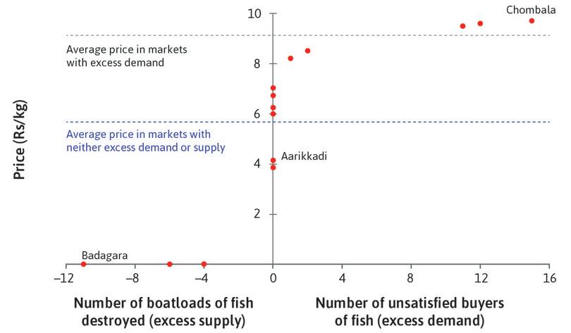
On 14 January 1997, for example, 11 boatloads of fish brought to the market at the town of Badagara found the market oversupplied, and jettisoned their catch. There was excess supply of 11 boatloads. But at fish markets within 15 km of Badagara there was excess demand: 15 buyers left the Chombala market unable to purchase fish at any price. The luck, or lack of it, of fishermen returning to the ports along the Kerala coast is illustrated in Figure 11.1.
- law of one price
- Holds when a good is traded at the same price across all buyers and sellers. If a good were sold at different prices in different places, a trader could buy it cheaply in one place and sell it at a higher price in another. See also: arbitrage.
Only seven of the 15 markets did not suffer either from over- or under-supply. In these seven villages (on the vertical line) prices ranged from Rs4 per kg to more than Rs7 per kg. This is an example of how the law of one price—a characteristic of a competitive market equilibrium—is sometimes a poor guide to how actual markets function.
Bargaining power and prices in the Kerala wholesale fish market (14 January 1997). (Note: Two markets had the same outcome, with a price of Rs4 per kg.)
Figure 11.1 Bargaining power and prices in the Kerala wholesale fish market (14 January 1997). (Note: Two markets had the same outcome, with a price of Rs4 per kg.)
Robert Jensen. 2007. ‘The Digital Provide: Information (Technology), Market Performance, and Welfare in the South Indian Fisheries Sector.’ The Quarterly Journal of Economics 122 (3) (August): pp. 879–924.
When the fishermen have bargaining power because there is excess demand, they get much higher prices. In markets with neither excess demand nor excess supply, the average price was Rs5.9 per kg, shown by the horizontal dashed line. In markets with excess demand, the average was Rs9.3 per kg. The fishermen fortunate enough to put in at these markets obtained extraordinary profits, if we assume that the price in markets with neither excess demand nor supply was high enough to yield economic profits. Of course, on the following day they may have been the unlucky ones who found no buyers at all, and so would dump their catch into the sea.
This all changed when the fishermen got mobile phones. While still at sea, the returning fishermen would phone the beach fish markets and pick the one at which the prices that day were highest. If they returned to a high-priced market they would earn an economic rent (that is, income in excess of their next best alternative, which would be returning to a market with no excess demand or even one with excess supply).
By gaining access to real-time market information on relative prices for fish, the fishermen could adjust their pattern of production (fishing) and distribution (the market they visit) to secure the highest returns.
A study of 15 beach markets along 225 km of the northern Kerala coast found that, once the fishermen used mobile phones, differences in daily prices among the beach markets were cut to a quarter of their previous levels. No boats jettisoned their catches. Reduced waste and the elimination of the dealers’ bargaining power raised the profits of fishermen by 8% at the same time as consumer prices fell by 4%.
Mobile phones allowed the fishermen to become very effective rent-seekers, and their rent-seeking activities changed how Kerala’s fish markets worked: they came close to implementing the law of one price, virtually eliminating the periodic excess demand and supply, to the benefit of fishermen and consumers (but not of the fish dealers who had acted as middlemen).
This happened because the Kerala sardine fishermen could respond to the information given by the prices at different beaches. It is another example of the idea we introduced in Unit 8 to explain the effect of the American Civil War on markets for cotton: that prices can be messages. For the economist Friedrich Hayek, this was the key to understanding markets.
Great economists Friedrich Hayek
The Great Depression of the 1930s ravaged the capitalist economies of Europe and North America, throwing a quarter of the workforce out of work in the US. During the same period, the centrally planned economy of the Soviet Union continued to grow rapidly under a succession of five-year plans. Even the arch-opponent of socialism, Joseph Schumpeter, had conceded:
‘Can socialism work? Of course it can … There is nothing wrong with the pure theory of socialism.’
Friedrich Hayek (1899–1992) disagreed. Born in Vienna, he was an Austrian (later British) economist and philosopher who believed that the government should play a minimal role in the running of society. He was against any efforts to redistribute income in the name of social justice. He was also an opponent of the policies advocated by John Maynard Keynes designed to moderate the instability of the economy and the insecurity of employment.
Hayek’s book The Road to Serfdom was written against the backdrop of the Second World War, when economic planning was being used both by German and Japanese fascist governments, by the Soviet communist authorities, and by the British and American governments. He argued that well-intentioned planning would inevitably lead to a totalitarian outcome.1
His key idea about economics revolutionized how economists think about markets. It was that prices are messages. They convey valuable information about how scarce a good is, but information that is available only if prices are free to be determined by supply and demand, rather than by the decisions of planners. Hayek even wrote a comic book, which was distributed by General Motors, to explain how this mechanism was superior to planning.
But Hayek did not think much of the theory of competitive equilibrium that we explained in Unit 8, in which all buyers and sellers are price-takers. ‘The modern theory of competitive equilibrium,’ he wrote, ‘assumes the situation to exist which a true explanation ought to account for as the effect of the competitive process.’
In Hayek’s view, assuming a state of equilibrium (as Walras had done in developing general equilibrium theory) prevents us from analysing competition seriously. He defined competition as ‘the action of endeavouring to gain what another endeavours to gain at the same time.’ Hayek explained:
Now, how many of the devices adopted in ordinary life to that end would still be open to a seller in a market in which so-called ‘perfect competition’ prevails? I believe that the answer is exactly none. Advertising, undercutting, and improving (‘differentiating’) the goods or services produced are all excluded by definition—’perfect’ competition means indeed the absence of all competitive activities. (The Meaning of Competition, 1946)
The advantage of capitalism, to Hayek, is that it provides the right information to the right people. In 1945, he wrote:
Which of these systems [central planning or competition] is likely to be more efficient depends mainly on the question under which of them we can expect [to make fuller use] of the existing knowledge. This, in turn, depends on whether we are more likely to succeed in putting at the disposal of a single central authority all the knowledge which ought to be used but which is initially dispersed among many different individuals, or in conveying to the individuals such additional knowledge as they need in order to enable them to dovetail their plans with those of others. (The Use of Knowledge in Society, 1945)
Hayek’s challenging ideas, and their application, are still fiercely debated today.2
- exogenous
- Coming from outside the model rather than being produced by the workings of the model itself. See also: endogenous.
- endogenous
- Produced by the workings of a model rather than coming from outside the model. See also: exogenous
Unit 8 introduced the concept of competitive market equilibrium, a situation in which the actions of the buyers and sellers of a good have no tendency to change its price, or the quantity traded, and the market clears. We saw that changes from the outside called exogenous shocks, like an increase in the demand for bread or a new tax, will alter the equilibrium price and quantity.
The opposite of exogenous is endogenous, meaning ‘coming from the inside’ and resulting from the workings of the model itself. In this unit, we will study how prices and quantities change through endogenous responses to exogenous shocks and the real-world competition that Hayek complained was absent from the model of competitive equilibrium. We will see that rent-seeking behaviour by market participants can bring about market clearing, move markets to different equilibria in the long run, cause bubbles and crashes, or lead to the development of secondary markets in response to price controls.
Question 11.1 Choose the correct answer(s)
Figure 11.1 shows how bargaining power affected prices in Kerala beach markets on 14 January 1997. Based on this information, what can we conclude?
- The price of fish is zero in all markets with excess supply.
- The average price in the markets with excess demand is 9.3, but the higher the excess demand, the higher the price.
- The law of one price is not satisfied because fish are sold at different prices in different places.
- When there is excess supply, the price is zero. The buyers have all the bargaining power while sellers have none.
11.1 How people changing prices to gain rents can lead to a market equilibrium
When Lincoln’s decision to blockade the southern ports led to a drastic shortage of cotton on the world market (Unit 8), people saw the opportunity to benefit by changing the price. In turn, these price changes sent a message to producers and consumers around the world to change their behaviour.
The blockade was an exogenous shock that changed the market equilibrium. In a competitive equilibrium, all trades take place at the same price (the market-clearing price), and buyers and sellers are price-takers. An exogenous shift in supply or demand means that the price has to change if the market is to reach the new equilibrium. The following example shows how this can happen.
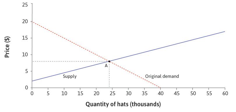
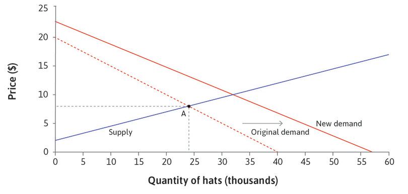
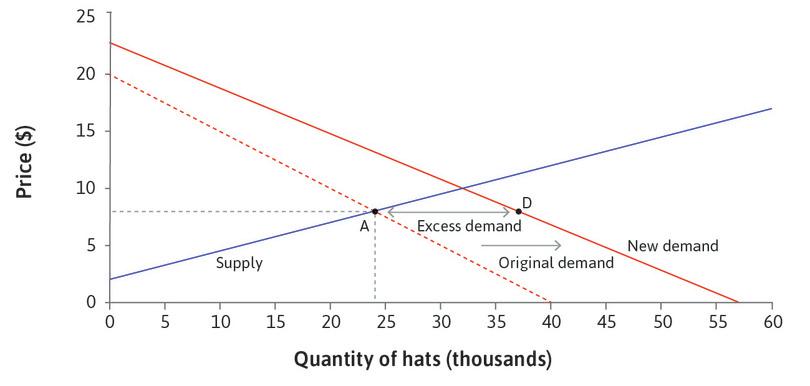
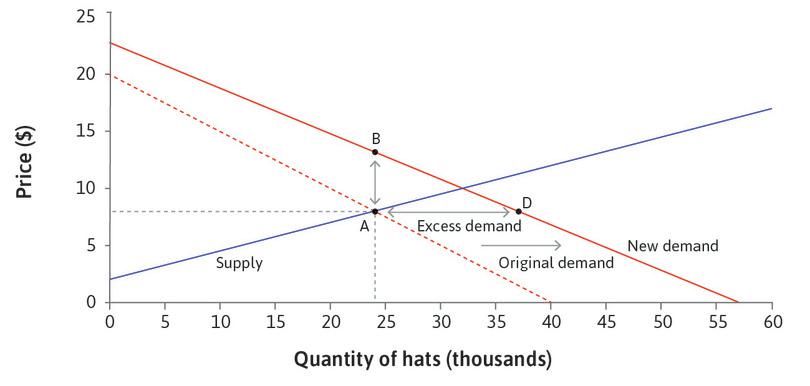
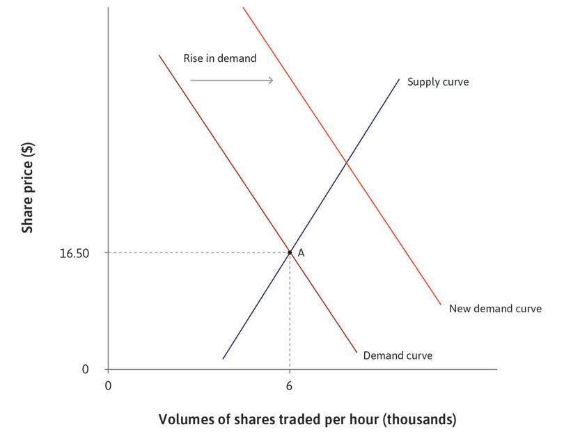
Figure 11.2 shows the competitive equilibrium in a market for hats. At point A, the equilibrium price equalizes the number of hats demanded by consumers to the number produced and sold by hat-sellers. At this point, no one can benefit by offering or charging a different price, given the price everyone else is offering or charging—it is a Nash equilibrium. Follow the steps in Figure 11.2 to see how an increase in the demand for hats gives hat-sellers an opportunity to benefit.
At the original point of competitive equilibrium (A) the price was $8, and all buyers and sellers were acting as price-takers. When demand increases, the buyers or sellers do not immediately know that the equilibrium price has risen to $10. If everyone were to remain a price-taker, the price would not change. But when demand shifts, some of the buyers or sellers will realize that they can benefit by being a price-maker, and decide to charge a different price from the others.
For example, when a hat-seller notices that every day there are customers wishing to buy hats, but none left on the shelf, she realizes that some customers would have been happy to pay more than the going price, and that some who paid the going price for their hat would have been willing to pay more. So the hat-seller will raise her price the next day—price-taking is no longer her best strategy, and she becomes a price-maker. She does not know exactly where the new demand curve is, but she cannot fail to see the people who want to buy hats go home disappointed.
By raising the price she raises her profit rate, and earns an economic rent (at least temporarily)—that is, she makes higher profits than are necessary to keep her hat business going. Moreover, because her price now exceeds her marginal cost, she will produce and sell more hats. The same is true of other hat-sellers who will experiment with higher prices and increased outputs.
As a result of the rent-seeking behaviour of hat-sellers, the industry adjusts to the new equilibrium at point C in Figure 11.2. At this point the market again clears, supply is equal to demand, and none of the sellers or buyers can benefit from charging a price different from $10. They all return to being price-takers, until the next change in supply or demand comes along.
When a market is not in equilibrium, both buyers and sellers can act as price-makers, transacting at a price different from the previous equilibrium price. If we start from the original equilibrium and take the opposite case of a fall in demand for hats, there will be excess supply at the going price of $8. A customer at the hat shop might say to the hat-seller: ‘I see you have quite a few unsold hats piling up on your shelf. I’d be happy to buy one of those for $7.’ To the buyer this would be a bargain. But it’s also a good deal for the seller, because at the reduced level of sales, $7 is still greater than the hat-seller’s marginal cost of producing the hat.
Market equilibration through rent-seeking
- disequilibrium rent
- The economic rent that arises when a market is not in equilibrium, for example when there is excess demand or excess supply in a market for some good or service. In contrast, rents that arise in equilibrium are called equilibrium rents.
The hats example illustrates how markets adjust to equilibrium through the pursuit of disequilibrium economic rents:
- When a market is in competitive equilibrium: If there is an exogenous change in demand or supply, there will be either excess demand or excess supply at the original price.
- Then, there are potential rents: Some buyers are willing to pay prices that are different from the original price, but above the marginal cost for the seller.
- While the market is in disequilibrium: Buyers and sellers can gain these rents by transacting at different prices. They become price-makers.
- This process continues until there is a new competitive equilibrium: At this point there is no excess demand or supply, and buyers and sellers are price-takers again.
- innovation rents
- Profits in excess of the opportunity cost of capital that an innovator gets by introducing a new technology, organizational form, or marketing strategy. Also known as: Schumpeterian rents.
Notice how market equilibration through rent-seeking resembles the process of technological improvement through rent-seeking modelled in Unit 2. There the exogenous change was the possibility of adopting a new technology. The first firm to do so gained innovation rents: profits in excess of the normal profit rate. This process went on until the innovation was widely diffused in the industry and prices had adjusted so that there were no further innovation rents to be had.
Einstein Equilibration through rent-seeking in an experimental market
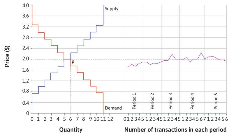
Economists have studied the behaviour of buyers and sellers in laboratory experiments to assess whether prices do adjust to equalize supply and demand. In the first such experiment, done in 1948, Edward Chamberlin gave each member of a group of Harvard students a card designating them as ‘buyers’ or ‘sellers’ and stating their willingness to pay or reservation price in dollars. They could then bargain amongst themselves, and he recorded the trades that took place. He found that prices tended to be lower, and the number of trades higher, than the equilibrium levels. Chamberlin would repeat the experiment every year. One of the students who took part in 1952, Vernon Smith, later conducted his own experiments and won a Nobel Prize in economics as a result.
He modified the rules of the game so that participants had more information about what was happening: buyers and sellers called out prices that they were willing to offer or accept. When anyone agreed to a proposed deal, a trade took place and the two participants dropped out of the market. His second modification was to repeat the game several times, with the participants keeping the same card in each round.
Figure 11.3 shows his results. There were 11 sellers, with reservation prices between $0.75 and $3.25, and 11 buyers with WTP in the same range. The diagram shows the corresponding supply and demand functions. You can see that, in equilibrium, six trades will take place at a price of $2. But the participants did not know this, since they did not know the price on anyone else’s card. The right-hand-side of the diagram shows the price for each trade that occurred. In the first period there were five trades, all at prices below $2. But by the fifth period most prices were very close to $2, and the number of trades was equal to the equilibrium quantity.
Vernon L. Smith. 1962. ‘An Experimental Study of Competitive Market Behavior’. Journal of Political Economy 70 (3) (January): p. 322.
Smith’s experiment provides some support for applying the model of competitive equilibrium to describe markets in which goods are identical–there are enough buyers and sellers, and they are well informed about the trading of others. The outcome was close to equilibrium even in the first period, and converged quickly towards it in subsequent periods as the participants learned more about supply and demand. The competitive model does not capture the rent-seeking behaviour during periods of adjustment in the experiment, but it correctly predicts the eventual outcome to be the price-taking equilibrium.
Exercise 11.1 A supply shock and adjustment to a new market
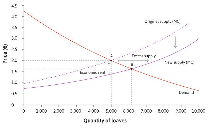
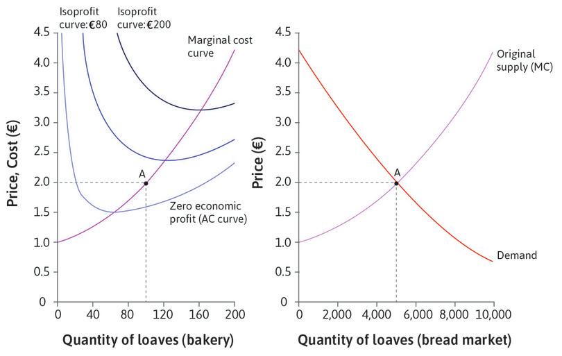
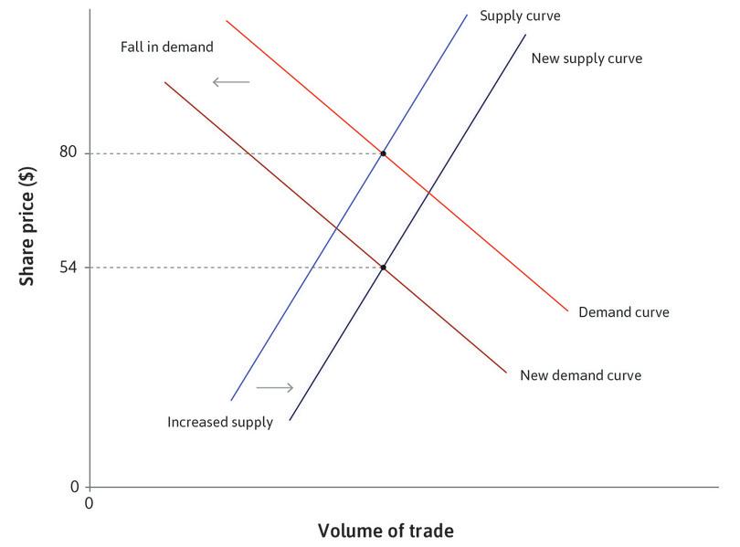
Consider a market in which bakeries supply bread to the restaurant trade. A new technology becomes available to the bakeries, shifting the supply curve as shown in the figure.
- Explain why the bakeries would want to increase sales. Why can they not do so at the original price?
- Describe how the actions of bakeries could adjust the industry to a new equilibrium.
- Is it always the seller who benefits from the economic rents that arise when the market is in disequilibrium?
- What action might restaurants take while the market is not in equilibrium?
Exercise 11.2 Cotton prices and the American Civil War
Read the introduction to Unit 8 and the ‘Great Economist’ box about Friedrich Hayek in this unit. Use the supply-and-demand model to represent:
- The increase in the price of US raw cotton (show the market for US raw cotton, a market with many producers and buyers).
- The increase in the price of Indian cotton (show the market for Indian raw cotton, a market with many producers and buyers).
- The reduction in textile output in an English textile mill (show a single firm in a competitive product market).
In each case, indicate which curve(s) shift and explain the result.
Question 11.2 Choose the correct answer(s)
Figure 11.2 shows the hat market before and after a demand shift. Based on this information, which of the following statements are correct?
- Sellers would not increase sales beyond A at $8, because their marginal cost would be higher than $8.
- Adjustment requires prices and quantities to be changed. rent-seeking provides incentives for buyers and sellers to make these changes.
- Until the new equilibrium is reached, buyers and sellers may find opportunities to benefit from transactions at different prices.
- In the new equilibrium, the law of one price holds and supply equals demand (at the new demand curve). The price will be $10.
11.2 How market organization can influence prices
Social interactions and market organization can both have a powerful impact on prices. Data from fish markets (which are good for comparison because fish are relatively homogeneous) show how influential both can be.
On the eastern coast of Italy, the Ancona fish market uses a Dutch auction system. When a crate of fish goes down a conveyor belt, a screen displays the initial price of the crate. That price declines incrementally until a seller pushes a button to buy the case. Transactions occur every four seconds on three active belts and €25 million of fish are sold annually. An auctioneer decides the initial prices, and buyers representing supermarkets and restaurants compete to determine final prices.
The Marseille fish market uses a different system. Sellers agree a price with each buyer who approaches their stand. This is called pairwise trading. If Paul is a seller, and buyer George approaches his stand to purchase a box of sardines, Paul offers him a price. That price may differ from the price Paul offers his next buyer. There is minimal haggling but George is free to reject a price and find another seller.
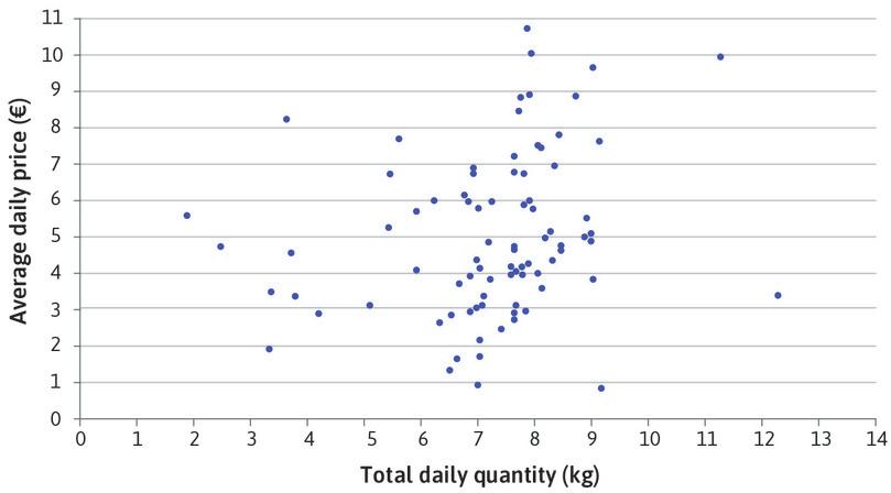
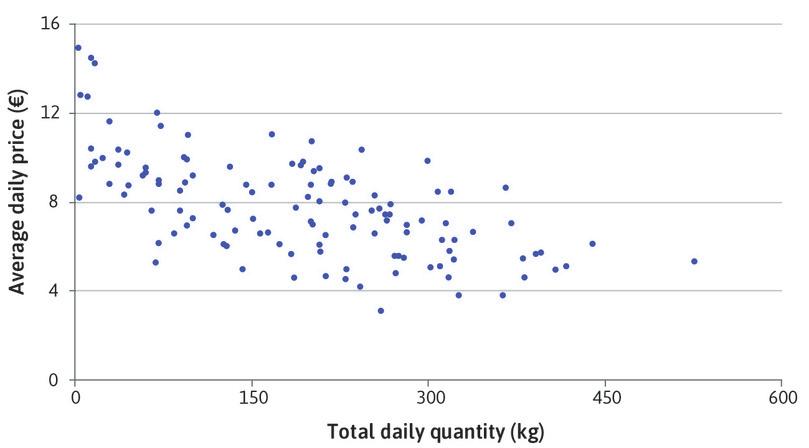
Some individual vendors in the Marseille market vary the prices of the same fish to different consumers by up to 30%. An individual buyer can end up paying very different amounts for different transactions of the same fish. Despite this, there is a typical downward-sloping relationship between price and quantity in the aggregate market.
- price discrimination
- A selling strategy in which different prices are set for different buyers or groups of buyers, or prices vary depending on the number of units purchased.
Alan Kirman used data on buyer loyalty to explain this kind of price discrimination. The Marseille market is composed of approximately 45 sellers and 500 buyers, many of whom are retailers like those in Ancona. Some buyers are extremely loyal to certain fishmongers, and others circulate. More loyal customers pay slightly higher prices than their less loyal counterparts. Kirman’s data reveal that this arrangement has led to higher profits for sellers and higher payoffs for 90% of loyal customers.
How does this make sense? Buyer payoffs come from both price and the satisfaction of demand. Imagine you are a buyer. On your first day at the Marseille market you are equally likely to buy from any of the fishmongers. You buy cod from Sarah and your supermarket makes a profit, making you more likely to return to Sarah next day. In this way, your past experiences inform your present decisions.
After continuing to buy from Sarah for some time, she begins serving you cod before her other customers as a reward for your loyalty. So you keep buying from Sarah because you are more likely to get all of the fish that you demand. The benefits of being a loyal customer are especially apparent when the weather limits the quantity of fish available.
Now imagine you are the fishmonger. Seller payoffs come from profits and the satisfaction of your supply. By increasing the number of loyal customers you have, your revenue becomes more reliable and your demand predictions become more accurate.
If you give loyal customers priority over others—perhaps by serving them first—you improve their experience buying from you, making them more likely to return. Over time these customers become so loyal that they will remain despite a small increase in the prices that you charge them.
In this manner, individual relationships and past experiences influence prices. The pairwise trading structure allows for customer loyalty to have a heavy influence on prices in the Marseille market.
Remarkably something very similar happens in Ancona, which has been studied by Mauro Gallegati and his co-authors. Figure 11.4 shows that some individual buyers in the market have very atypical price-quantity relationships. But as shown in Figure 11.5, the aggregate price quantity relationship is standard. Even without face-to-face interaction, buyer loyalty is present and some consumers are more likely to buy from certain ships. Unlike the Marseille market, however, many of these loyal customers pay lower prices than their less loyal counterparts. This is puzzling, since there is no face-to-face contact between buyers and sellers. The authors believe that this is due to a complex learning process.
Another noteworthy fact about the Ancona market is that prices fall during the day. In this case, why don’t buyers simply wait for better prices? Once again we must consider a trade-off—if buyers wait until later in the day, it becomes more likely that they will not be able to buy the fish that they want. Many buyers may not be willing to accept that risk and will pay higher prices to guarantee that they get their fish. Consistent with this explanation, prices rise sharply at the end of the day when total supply is low.
Prices ultimately come from the interests of and relationships between buyers and sellers. Market organization determines precisely how these relationships influence prices.
The price-quantity relationship for a single buyer in the Ancona fish market.
Figure 11.4 The price-quantity relationship for a single buyer in the Ancona fish market.
Mauro Gallegati, Gianfranco Giulioni, Alan Kirman, and Antonio Palestrini. 2011. ‘What’s that got to do with the price of fish? Buyers behavior on the Ancona fish market’. Journal of Economic Behavior & Organization 80 (1) (September): pp. 20–33.
The aggregate price-quantity relationship in the Ancona market.
Figure 11.5 The aggregate price-quantity relationship in the Ancona market.
Mauro Gallegati, Gianfranco Giulioni, Alan Kirman, and Antonio Palestrini. 2011. ‘What’s that got to do with the price of fish? Buyers behavior on the Ancona fish market’. Journal of Economic Behavior & Organization 80 (1) (September): pp. 20–33.
11.3 Short-run and long-run equilibria
When we modelled equilibrium in the market for bread in Unit 8, we assumed that there were a fixed number of bakeries (50) in the city. We worked out the industry supply curve by adding together the amounts of bread each bakery would supply at each price, and then found the equilibrium price and quantity.
But we also saw that at the equilibrium price, the bakeries were earning rents (their economic profits were greater than zero), providing an opportunity for other firms to benefit by entering the market. Entry of new firms would shift market supply, leading to a new equilibrium. This is an example of how rent-seeking can move a market to a different equilibrium in the long run.
- short-run equilibrium
- An equilibrium that will prevail while certain variables (for example, the number of firms in a market) remain constant, but where we expect these variables to change when people have time to respond to the situation.
- long-run equilibrium
- An equilibrium that is achieved when variables that were held constant in the short run (for example, the number of firms in a market) are allowed to adjust, as people have time to respond the situation.
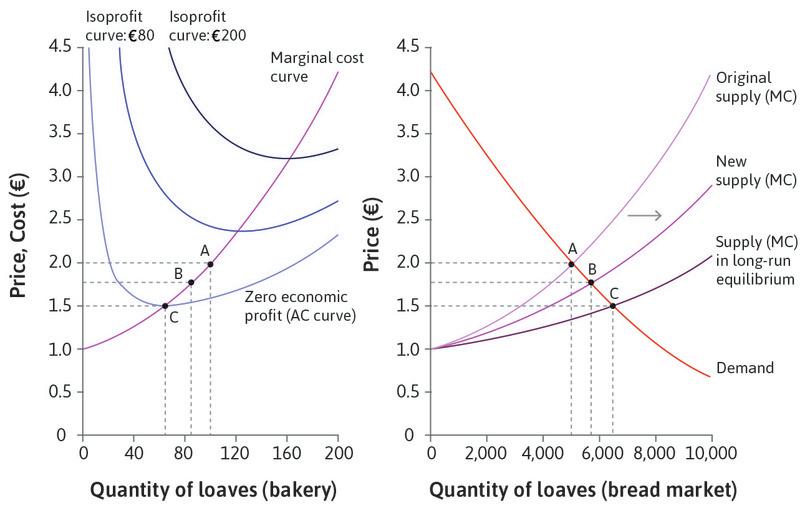
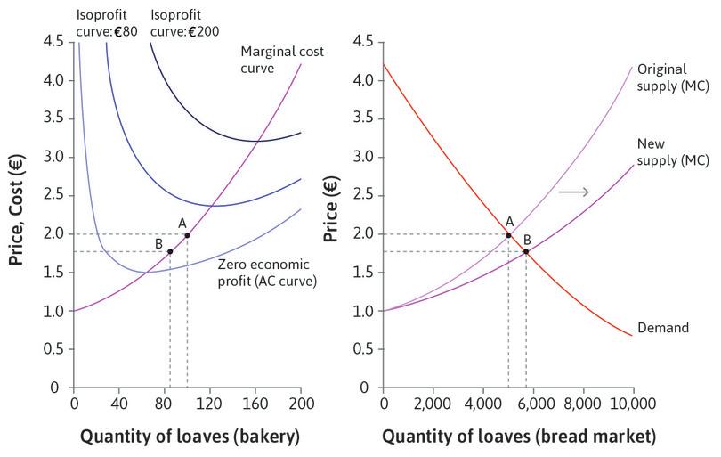
Figure 11.6 shows the bread market equilibrium with 50 bakeries at point A in the right-hand panel: 5,000 loaves are sold at €2 each. The left-hand panel shows the isoprofit and marginal cost curves for each bakery (assuming they are identical) and the point where it produces when the price is €2: it produces 100 loaves (where price equals marginal cost). And we can see that at point A it is above the average cost curve, earning a positive economic profit.
The market equilibrium at point A is described as a short-run equilibrium. The phrase ‘short-run’ is used to indicate that we are holding something constant for now, although it might change in future. In this case, we mean that point A is the equilibrium while the number of firms in the market remains constant. But because firms are earning rents, we do not expect this situation to last. Follow the steps to see what happens in the longer run.
When the long-run equilibrium is reached at point C, the price of bread is equal to both the marginal and the average cost (P = MC = AC), and every bakery’s economic profit is zero.
In the long run, profits to be made in the bread market are no higher than the profits that potential bakery owners could make by using their assets elsewhere. And, if any owners could do better by putting their premises to a different use (or by selling them and investing in a different business) we would expect them to do so. Although no one would be earning more than normal profits, no one should be earning less than normal profits either.
We can use Figure 11.6 to work out how many bakeries there will be in the long-run equilibrium. The left-hand panel shows that the price must be €1.52, because that is the point on the firm’s supply curve where the firm makes normal profits (P = MC = AC), and each bakery produces 66 loaves. From the demand curve in the right-hand panel, we can deduce that at this price the quantity of bread sold will be 6,500 loaves. So the number of bakeries in the market must be 6,500/66 = 98.
Notice how the short-run and long-run equilibrium differ. In the short run, the number of firms is exogenous—it is assumed to remain constant at 50. In the long run, the number of bakeries can change through the endogenous rent-seeking responses of firms. The number of firms in the long-run equilibrium is endogenous—it is determined by the model.
The concepts of short- and long-run equilibria don’t have much to do with specific periods of time, except that some variables (such as the market price and the quantity produced by individual firms) can adjust more quickly than others (such as the number of firms participating in a market). So what we mean by the short run and the long run depends on the model. The short-run equilibrium is achieved when everyone has done the best they can from adjusting the easily adjustable variables while the others remain constant. The long-run equilibrium happens when these other variables have adjusted too.
Short-run and long-run elasticities
Remember from Unit 8 that when demand for a good increases, the increase in the quantity sold depends on the elasticity of the supply curve (that is, the marginal cost curve). So if the demand for bread increases, a steep (inelastic) supply curve means that the price of bread rises a lot in the short run while the number of bakeries is fixed, with a relatively small rise in quantity. But in the longer run, this will lead to more bakeries entering, so the price falls, and quantity increases more. We say that, because of the possibility of entry and exit of firms, the supply of bread is more elastic in the long run.
The distinction between the short run and the long run applies in many economic models. Besides the number of firms in an industry, there are lots of other economic variables that adjust slowly, and it is useful to distinguish between what happens before and after they adjust.
In the next section, we will see another example: both the supply and the demand for oil are more elastic in the long run, because producers can eventually build new oil wells, and consumers can switch to different fuels for cars or heating. What we mean by the short run in this case is the period during which firms are limited by their existing production capacity, and consumers by the cars and heating appliances they currently own.
Question 11.3 Choose the correct answer(s)
Figure 11.6 shows the market for bread in the short run, with 50 bakeries, and in the long run when more bakeries can enter. All bakeries are identical. Which of the following statements is correct?
- The supply curve of each bakery remains the same. It is the market supply curve that shifts.
- A and B can only be short-run equilibria, for a given number of bakeries. The economic rent will encourage more bakeries to enter.
- No more bakeries will enter because the price would then fall below average cost and they would make a loss.
- At C the bakeries are making normal profits, so there is no reason to leave.
11.4 Prices, rent-seeking, and market dynamics at work: Oil prices
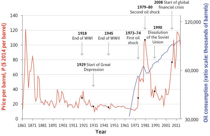
Figure 11.7 plots the real price of oil in world markets (in constant 2014 US dollars) and the total quantity consumed globally from 1865 to 2014. To understand what drives the large fluctuations in the oil price, we can use our supply and demand model, distinguishing between the short run and the long run.
World oil prices in constant prices (1865–2014) and global oil consumption (1965–2014).
Figure 11.7 World oil prices in constant prices (1865–2014) and global oil consumption (1965–2014).
BP. (2015) BP Statistical Review of World Energy June 2015.
We know that prices reflect scarcity. If a good becomes scarcer, or more costly to produce, the supply will fall and price will tend to rise. For more than 60 years, oil industry analysts have been predicting that demand would soon outstrip supply: production would reach a peak and prices would then rise as world reserves declined. ‘Peak oil’ is not evident in Figure 11.7. One reason is that rising prices provide incentives for further exploration. Between 1981 and 2014, more than 1,000 billion barrels were extracted and consumed, yet world reserves of oil more than doubled from roughly 680 billion barrels to 1,700 billion barrels.
Prices have risen strongly in the twenty-first century and an increasing number of analysts are predicting that conventional oil, at least, has reached a peak. But unconventional resources such as shale oil are now being exploited. Perhaps it will be climate change policies, rather than resource depletion, that eventually curb oil consumption.3 4
What makes the price messages in Figure 11.7 hard to read is the sharp swings from high to low and back again over short periods of time. These fluctuations cannot be explained by looking at oil reserves, because they reflect short-run scarcity. Both supply and demand are inelastic in the short run.
Short-run supply and demand
On the demand side, the main use of oil products is in transport services (air, road, and sea). Demand is inelastic in the short run because of the limited substitution possibilities. For example, even if petrol prices rise substantially, in the short run most commuters will continue to use their existing cars to travel to work because of the limited alternatives immediately available to them. So the short-run demand curve is steep.
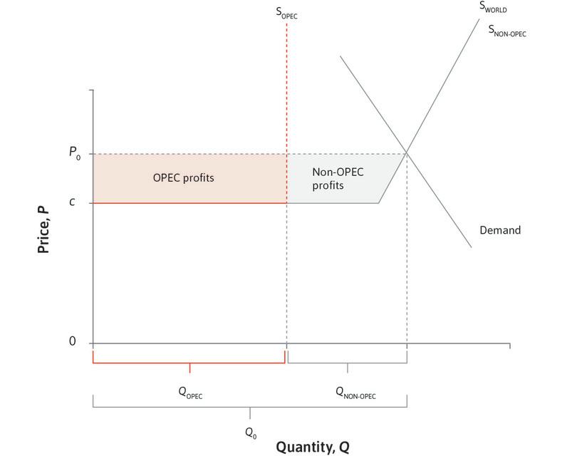
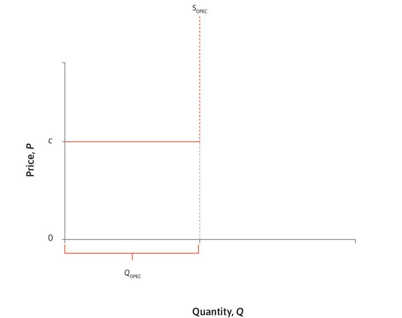
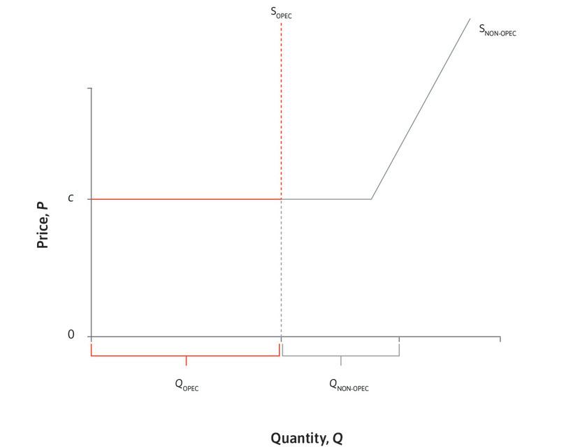
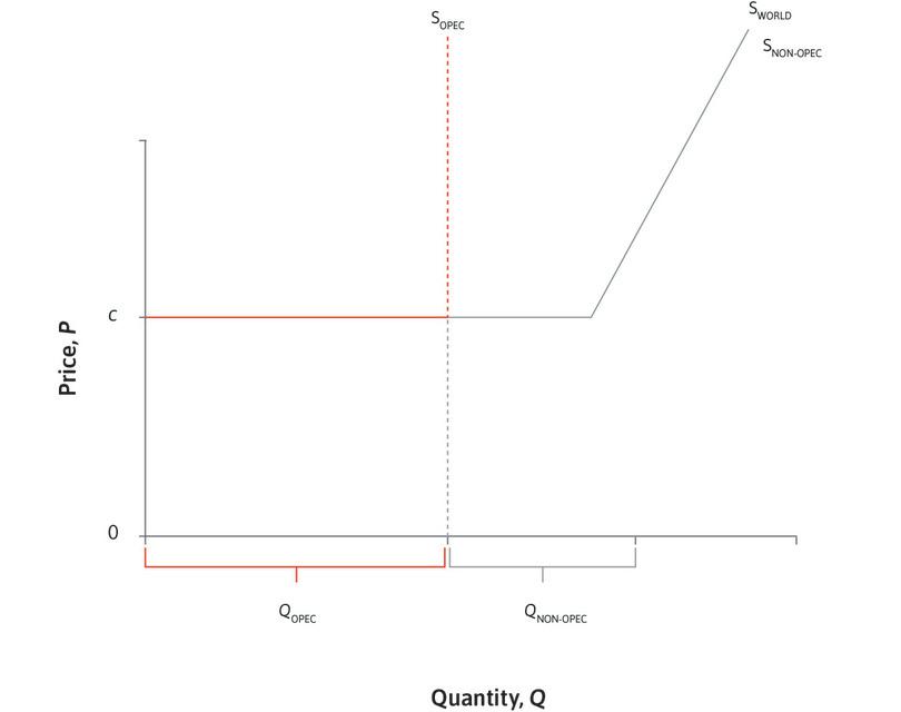
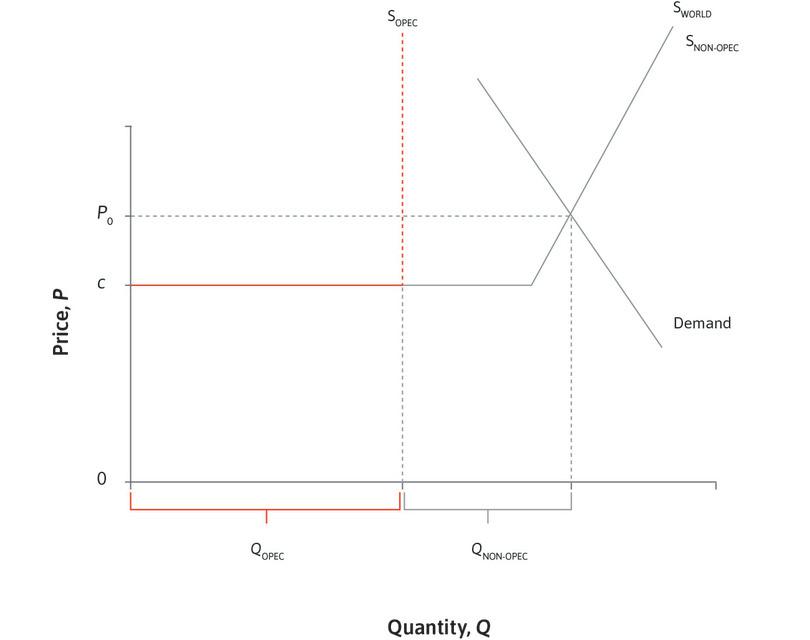
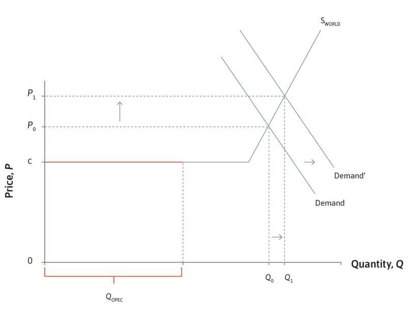
Traditional oil extraction technology is characterized by a large up-front investment in expensive oil wells that can take many months or longer to construct, and once in place, can keep pumping until the well is depleted or oil can no longer be profitably extracted. Once the well is drilled, the cost of extracting the oil is relatively low, but the rate at which the oil is pumped faces capacity constraints—producers can get only so many barrels per day from a well. This means that, taking existing capacity as fixed in the short run, we should draw a short-run supply curve that is initially low and flat, and then turns upwards very steeply as capacity constraints are hit. We also need to allow for the oligopolistic structure of the world market for crude oil. The Organization of Petroleum Exporting Countries (OPEC) is a cartel with a dozen member countries that currently accounts for about 40% of world oil production. OPEC sets output quotas for its members. We can represent this in our supply and demand diagram by a flat marginal cost line that stops at the total OPEC production quota. At that point, the line becomes vertical. This is not because of capacity constraints, but because OPEC producers will not sell any more oil.
- oligopoly
- A market with a small number of sellers, giving each seller some market power.
Figure 11.8 assembles the market supply curve by adding the OPEC production quota to the non-OPEC supply curves (remember we obtain market supply curves by adding the amounts supplied by each producer at each price) and combines it with the demand curve to determine the world oil price.
The 1970s oil price shocks
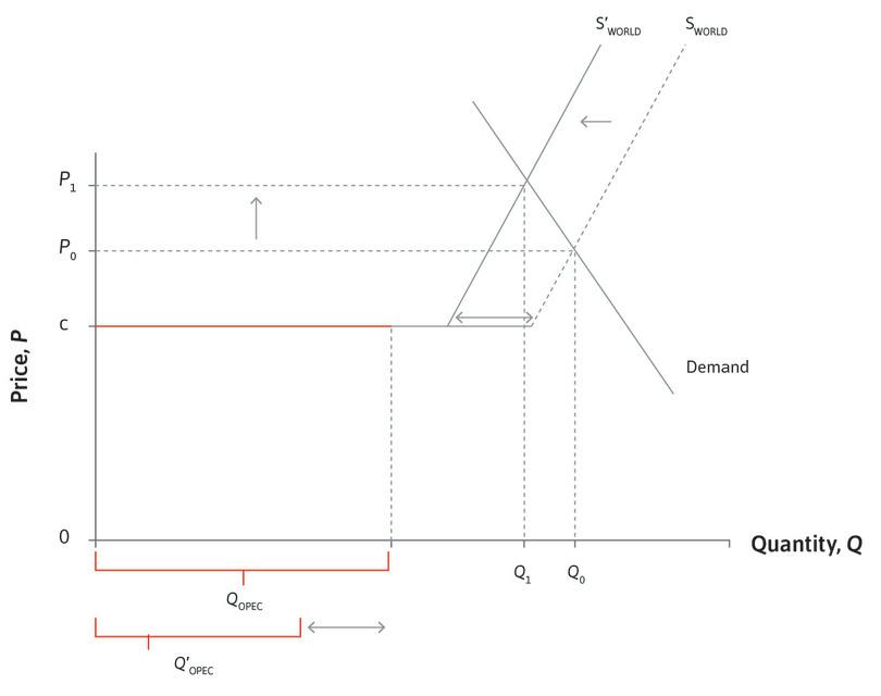
In 1973 and 1974, OPEC countries imposed a partial oil embargo in response to the 1973–4 Middle East war, and in 1979 and 1980, oil production by Iran and Iraq fell because of the supply disruptions following the Iranian Revolution and the outbreak of the Iran–Iraq war. These are represented in Figure 11.9 by a leftward shift of the world supply curve Sworld, driven by a reduction in the volume of OPEC production to Q′OPEC. Total production and consumption falls, but because demand is very price-inelastic, the percentage increase in price is much larger than the percentage decrease in quantity. This is what we see in the data in Figure 11.7. The oil price (in 2014 US dollars) goes from $18 per barrel in 1973 to $56 in 1974, and then to $106 in 1980, but the declines in world oil consumption after these price shocks are small by comparison (–2% between 1973 and 1975, and –10% between 1979 and 1983).
The 2000–2008 oil price shock
- income elasticity of demand
- The percentage change in demand that would occur in response to a 1% increase in the individual’s income.
The years 2000 to 2008 were a period of rapid economic growth in industrializing countries, especially China and India. The income elasticity of demand for oil and oil products is higher in these countries than in developed market economies, and demand for car ownership and tourist air travel is growing relatively rapidly as they become wealthier. This increase in income moves the demand curve to the right, as shown in Figure 11.10. In this case, it is the inelastic short-run supply curve for oil that accounts for the big increase in price and only a modest increase in world oil consumption. The sharp price decrease in 2009 has the same explanation but in reverse: the financial crisis of 2008–9 was a negative demand shock that moved the demand curve to the left, so world consumption fell by about 3%, and the price of crude fell from over $100 per barrel in the summer of 2008 to $40–50 in early 2009.
Exercise 11.3 The world market for oil
Using the supply and demand diagram:
- Illustrate what happens when economic growth boosts world demand
- in the short run
- in the long run as producers invest in new oil wells
- in the long run as consumers find substitutes for oil
- Similarly, describe the short and long-run consequences of a negative supply shock similar to the 1970s shock.
- If you observed an oil price rise, how in principle could you tell whether it was driven by supply-side or demand-side developments?
- How would the diagram, and the response to shocks, be different if there were:
- a competitive market composed of many producers?
- a single monopoly oil producer?
- an OPEC cartel controlling 100% of world oil production and seeking to maximize the combined profits of its members?
- Why would individual OPEC member countries have an incentive to produce more than the quota assigned to them?
- Does this logic carry over to the situation in the real world where there are also non-OPEC producers?
Exercise 11.4 The shale oil revolution
An important development in the past 10 years has been the re-emergence of the US as a major oil producer via the ‘shale oil revolution’. Shale oil is extracted using the technology of hydraulic fracturing or ‘fracking’: injecting fluid into ground at high pressure to fracture the rock and allow extraction. In a speech called ‘The New Economics of Oil’ in October 2015, Spencer Dale, group chief economist at oil producer BP plc, explained how shale oil production differs from traditional extraction.
- According to Dale, how has the shale oil revolution affected the world market for oil?
- How will the world oil market be different in future?
- Explain how our supply and demand diagram should be changed if his analysis is correct.
11.5 The value of an asset: Basics
- asset
- Anything of value that is owned. See also: balance sheet, liability.
People buy fish, hats, and fuel for their consumption value: to eat, wear, or burn them (respectively). Markets for assets can work differently because buyers have a second motive: not only to benefit in some way while owning the asset, but also to be able to sell it later. So what determines the value of an asset, whether it is real estate, an artwork, or a financial asset, such as shares in a firm?
Remember from Unit 6 that the profits of a firm belong to its shareholders in direct proportion to the shares that each holds. These profits are typically divided between dividends paid directly to shareholders, and retained earnings used to maintain and expand the firm’s ability to generate revenues. But since the future is so uncertain, how should these shares be valued?
Two important determinants of the value of a financial asset (also called a security) are the size of the cash flows that it is expected to generate, and uncertainty in one’s forecasts of these cash flows.
Bonds
- government bond
- A financial instrument issued by governments that promises to pay flows of money at specific intervals.
It is easiest to start with an asset that promises a fixed stream of payments at specified dates over a finite period. Suppose investors are completely confident that the promised payments will be made. The best example of this is a government bond issued by a country with a negligible likelihood of default, such as the US or Switzerland (this case was analysed in the Einstein in Unit 10).
- bond
- A type of financial asset for which the issuer promises to pay a given amount over time to the holder. Also known as: corporate bonds.
Investors will be willing to buy and hold the asset only if its rate of return—the future payments relative to the price at which it can be bought or sold—compares well with interest rates on similar assets elsewhere in the economy. The promised stream of payments is fixed, so the lower the price of the asset, the greater will be the interest rate that it yields to a buyer. In other words, the price of the asset will be inversely related to the interest rate that the asset yields. If other interest rates in the economy rise, the interest rate on bonds will have to rise too—so the price of bonds will fall.
Now consider corporate bonds, which are not risk-free. The greater the risk of default, the higher will be the interest rate that investors demand in order to hold the asset. If two bonds promise exactly the same stream of payments, the riskier one will have a lower price. Investors will earn a higher interest rate if they buy the riskier bond and it happens not to default, but face a greater risk that the promised payments will not all materialize.
Stocks
- share
- A part of the assets of a firm that may be traded. It gives the holder a right to receive a proportion of a firm’s profit and to benefit when the firm’s assets become more valuable. Also known as: common stock.
Stocks (also called shares) differ from bonds in two important respects: there is no specific promised stream of payments, and the time period over which payments will be made is not fixed. Firms expected to generate greater net earnings will have higher valuations, and if expectations change, so will the value of the shares. But like bonds, their value will also depend on interest rates elsewhere in the economy, and on how risky the earnings are thought to be.
Risk
- systematic risk
- A risk that affects all assets in the market, so that it is not possible for investors to reduce their exposure to the risk by holding a combination of different assets. Also known as: undiversifiable risk.
- idiosyncratic risk
- A risk that only affects a small number of assets at one time. Traders can almost eliminate their exposure to such risks by holding a diverse portfolio of assets affected by different risks. Also known as: diversifiable risk.
But how should the risk of an asset be assessed? Answering this question requires us to understand the distinction between systematic risk and idiosyncratic risk. The earnings of a firm may rise above or fall short of expectations for various reasons. Some events—such as changes in trade policy, interest rates, or economy-wide demand for goods and services —simultaneously affect broad classes of financial assets. Other events—such as a successful drug trial, or lawsuit alleging safety problems for a vehicle—affect only the specific firms that stand to lose or gain. The first source of risk is called systematic or undiversifiable, the second idiosyncratic or diversifiable.
- systemic risk
- A risk that threatens the financial system itself.
A third type of risk, systemic risk, usually refers to risks that threaten the financial system itself. We will examine examples of systemic risk, such as the 2008 financial crisis, in Unit 17.
This insight was developed by William Sharpe, John Lintner, and others in the 1960s, building on prior work by Harry Markowitz.
An important insight in the economics of finance is that diversifiable risk is essentially irrelevant in the valuation of securities, because investors can almost eliminate it by constructing portfolios that contain a large number of assets, each of which has a very small weight. In any given period some of the firms in the portfolio will experience positive shocks, and some negative, but as long as shocks are truly idiosyncratic, they will tend to cancel each other out and the portfolio itself will be largely unaffected.
Systematic risk is different. It arises from shocks that affect large classes of securities simultaneously and cannot be diversified away. Different firms are exposed to different levels of systematic risk, depending on the degree to which their earnings are correlated with those of the market as a whole. For example, the earnings of Ford or Chrysler are heavily dependent on economic conditions in the economy as a whole, since people postpone purchases of cars during economic downturns. In contrast, utility companies providing gas and electricity to residential customers are sheltered from such risks since energy consumption is not very sensitive to economic conditions.
- market capitalization rate
- The rate of return that is just high enough to induce investors to hold shares in a particular company. This will be high if the company is subject to a high level of systematic risk.
Investors will demand higher average returns from shares in companies with high levels of systematic risk, since their earnings will tend to be volatile in ways that cannot be easily diversified away. The rate of return that will induce investors to buy shares in a company is sometimes called the required rate of return, or the market capitalization rate. Ceteris paribus, this rate will be higher for companies subject to greater systematic risk. So for any given beliefs about expected future earnings, share values will be higher for companies with lower market capitalization rates.
Trading strategies
- fundamental value of a share
- The share price based on anticipated future earnings and the level of systematic risk, which can be interpreted as a measure of the benefit today of holding the asset now and in the future.
The share price computed from such considerations—anticipated future earnings and the level of systematic risk—is sometimes called the fundamental value of a share or security. Many institutional investors, including actively managed mutual funds and some hedge funds, adopt trading strategies based on buying assets that they perceive to be priced below their fundamental values, and selling those that are overpriced relative to fundamentals.
However, there are other trading strategies that are not based on an assessment of fundamental value at all. For instance, some traders look for evidence of momentum in asset prices, buying because they expect prices to rise further, or selling because they expect prices to fall. An investor might be willing to pay more than the fundamental value of a security if she believes that the price will rise even further above this value. In this case, the buyer could make a gain by buying at a low price and selling at a higher price, even if the fundamental value of the security had not changed.
- speculation
- Buying and selling assets in order to profit from an anticipated change in their price.
Buying and selling assets based on an assessment of their fundamental values is a form of speculation, motivated by a belief that prices will soon return to their fundamental values. Buying and selling based on perceived momentum is also an example of speculation, motivated by a belief that short-run trends have a degree of persistence. These strategies, and many others, are present in modern financial markets. They determine the behaviour of prices, and the possibility of bubbles and crashes (as we shall see in later sections).
How economists learn from facts The wisdom of crowds: The weight of stock (oxen) and the value of stocks
What is the right price for, say, a share in Facebook? Would it be better for the price to be set by economic experts, rather than determined in the market by the actions of millions of people, few of whom have expert knowledge about the economy or the company’s prospects?
Economists are far from understanding the details of how this mechanism actually works. But an important insight comes from an unusual source: a guessing game played in 1907 at an agricultural fair in Plymouth, England. Attendees at the fair were presented with a live ox. For sixpence (2.5p), they could guess the ox’s ‘dressed’ weight, meaning how much saleable beef could be obtained. The entrant whose answer written on a ticket came closest to the answer would win the prize.
The polymath Francis Galton later obtained the tickets associated with that contest. He found that a player chosen at random missed the correct weight by an average of 40 lbs. But what he called the ‘vox populi’ or ‘voice of the people’—the median value of all the guesses—was remarkably close to the true value, deviating by only 9 lbs (less than 1%).
The insight that is relevant to economics is that the average of a large number of not-very-well-informed people is often extremely accurate. It is possibly more accurate than the estimate of an experienced veterinarian or ox breeder.
Galton’s use of the median to aggregate the guesses meant that vox populi was the voice of the (assumed) most informed player but it was the guesses of all the others that picked out this most informed player. Vox populi was obtained by taking all of the information available, including the hunches and fancies that drove outliers high or low.
Galton’s result is an example of the ‘Wisdom of the Crowd’. This concept is particularly interesting for economists because it contains, in a stylized format, many of the ingredients that go into a good price mechanism.
As Galton himself noted, the guessing game had a number of features contributing to the success of vox populi. The entry fee was small, but not zero, allowing many to participate, but deterring practical jokers. Guesses were written and entered privately, and judgements were uninfluenced ‘by oratory and passion’. The promise of a reward focused the attention.
Although many participants were well informed, many were less so and, as Galton noted, were guided by others at the fair and their imagination. Galton’s choice of the median value would reduce (but not eliminate) the influence of these less-informed guessers, preventing individual wild guesses (say, those 10 times the true value) from pulling the vox populi away from the views of the group as a whole.
The stock market represents another expression of vox populi, where people guess at the value of a company, often but not always quite accurately tracking changes in the quality of management, technology, or market opportunities.
The wisdom of crowds also explains the success of prediction markets. The Iowa Electronic Markets, run by the University of Iowa, allows individuals to buy and sell contracts that pay off depending on who wins an upcoming election. The prices of these assets pool the information, hunches, and guesses of large numbers of participants. Such prediction markets–often called political stock markets—can provide uncannily accurate forecasts of election results months in advance, sometimes better than polls and even poll-aggregation sites. Other prediction markets allow thousands of people to bet on such events as who will win the Oscar for best female lead. It was even proposed to create a prediction market for the next occurrence of a major terrorist attack in the US.
Question 11.4 Choose the correct answer(s)
Which of the following statements is correct?
- Expected future profits and systematic risk determine the stream of income an investor can expect. This is what we mean by the fundamental value.
- With no new information about profitability or risk, the fundamental value has not changed, so a rising price indicates speculation.
- It is possible to benefit from this strategy if you sell before the price falls.
- Investors do not necessarily agree, since they may have different information about future profitability.
11.6 Changing supply and demand for financial assets
- stock exchange
- A financial marketplace where shares (or stocks) and other financial assets are traded. It has a list of companies whose shares are traded there.
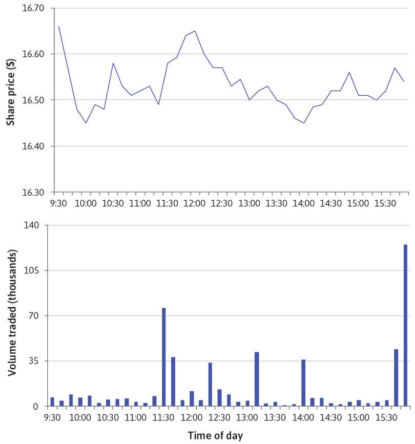
Prices in financial markets are constantly changing. The graph in Figure 11.11 shows how News Corp’s (NWS) share price on the Nasdaq stock exchange fluctuated over one day in May 2014 and, in the lower panel, the number of shares traded at each point. Soon after the market opened at 9.30 a.m., the price was $16.66 per share. As investors bought and sold shares through the day, the price reached a low point of $16.45 at both 10 a.m. and 2 p.m. By the time the market closed, with the share price at $16.54, nearly 556,000 shares had been traded.
News Corp’s share price and volume traded (7 May 2014).
Figure 11.11 News Corp’s share price and volume traded (7 May 2014).
Bloomberg L.P., accessed 28 May 2014.
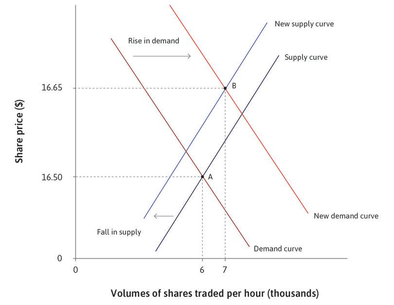
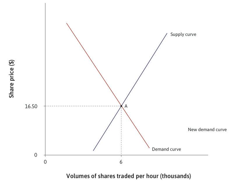
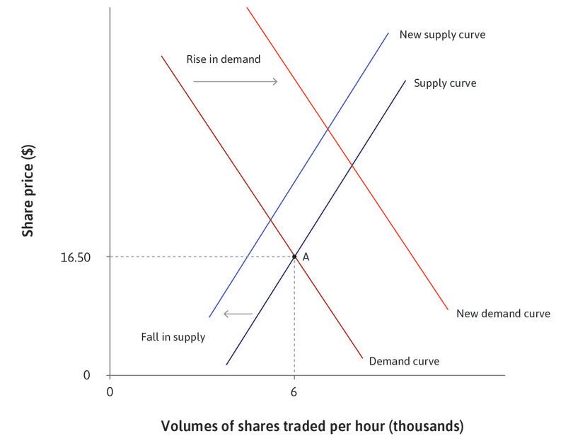
At any time when the market for shares in News Corp is open, each of the existing shareholders has a reservation price, namely the least price at which the shareholder would be willing to sell. Others are in the market to buy, as long as they can find an acceptable price. As traders’ beliefs about the profitability of News Corp change, their willingness to buy and sell changes. To see how the prices of financial assets are affected by such shifts in demand and supply, follow the steps in Figure 11.12. The curves show the hourly volume of shares that would be demanded and supplied at each price.
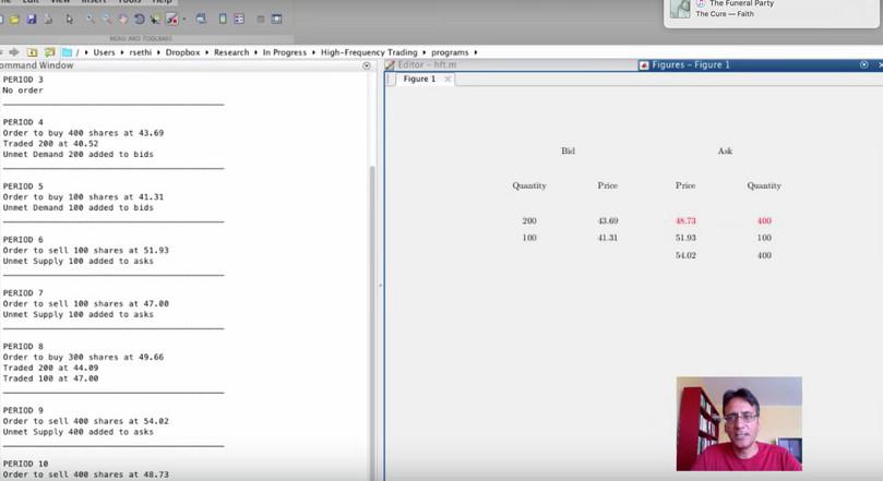
In practice, stock markets don’t operate in fixed time periods, such as an hour. Trade takes place continuously and prices are always changing, through a trading mechanism known as a continuous double auction.
- limit order
- An announced price and quantity combination for an asset, either to be sold or bought.
- order book
- A record of limit orders placed by buyers and sellers, but not yet fulfilled.
Anyone wishing to buy can submit a price and quantity combination known as a limit order. For instance, a limit order to buy 100 shares in News Corp at a price of $16.50 per share indicates that the buyer commits to buying 100 shares, as long as they can be obtained at a price no greater than $16.50 per share. This is the buyer’s reservation price. Similarly, a limit sell order indicates a commitment to sell a given quantity of shares, as long as the price is no less than the amount specified (the seller’s reservation price).
When a limit buy order is placed, one of two things can happen. If a previously placed limit sell order exists that has not yet been filled, and it offers the required number of shares at a price that is at or below the amount indicated by the buyer, a trade occurs. If there is no such order available, then the limit order is placed in what is called an order book (which is really just an electronic record), and becomes available to trade against new sell orders that arrive.
Orders to buy are referred to as bids, and orders to sell as asks. The order book lists bids in decreasing order of price, and asks in increasing order. The top of the book for shares in NWS at around midday on 8 May 2014 looked like the table in Figure 11.13.
| Bid | Ask | ||
|---|---|---|---|
| Price ($) | Quantity | Price ($) | Quantity |
| 16.56 | 400 | 16.59 | 500 |
| 16.55 | 400 | 16.60 | 700 |
| 16.54 | 400 | 16.61 | 800 |
| 16.53 | 600 | 16.62 | 500 |
| 16.52 | 200 | 16.63 | 500 |
A continuous double auction order book: Bid and ask prices for News Corp (NWS) shares.
Figure 11.13 A continuous double auction order book: Bid and ask prices for News Corp (NWS) shares.
Yahoo Finance, accessed 8 May 2014.
Given this situation, a buy order for 100 shares at $16.57 would remain unfilled and would enter the book at the top of the bid column. However, a bid for 600 shares at $16.60 would be filled immediately, since it can be matched against existing limit sell orders. 500 shares would trade at $16.59 apiece, and 100 shares would trade at $16.60. Whenever a buy order is immediately filled, trade occurs at the best possible price for the buyer (the ask price). Similarly, if a sell order is placed and immediately filled from existing orders, trade occurs at the best possible price for the seller (the bid price).
We can now see how prices in such a market change over time. Someone who receives negative news about News Corp, such as a rumour that a board member is about to resign, and believes this information has not yet been incorporated into the price, may place a large sell order at a price below $16.56, which will immediately trade against existing bids. As these trades occur, bids are removed from the order book and the price of the stock declines. Similarly, in response to good news, orders to buy at prices above the lowest ask will trade against existing sell orders, and transactions will occur at successively increasing prices.
Since the price fluctuates, it is not easy to think of this market as being in equilibrium. But it is nevertheless the case that the price is always adjusting to reconcile supply and demand and hence clear the market.
Financial assets provide another example of markets equilibrating through economic rent-seeking:
- Those who believe they will benefit from buying News Corp shares at a particular price lodge a bid at that price.
- Those who believe they will benefit by selling lodge an ask at a particular price.
- The price at any moment reflects the aggregate outcome of the rent-seeking behaviour of all the actors in the market—including those who are simply holding on to their shares.
Exercise 11.5 Supply and demand curves
- Use the data from the NWS order book in Figure 11.13 to plot supply and demand curves for shares.
- Explain why the two curves do not intersect.
Question 11.5 Choose the correct answer(s)
The figure shows an order book for News Corp shares. Which of the following statements about this order book is correct?
| Bid | Ask | ||
|---|---|---|---|
| Price ($) | Quantity | Price ($) | Quantity |
| 16.56 | 400 | 16.59 | 500 |
| 16.55 | 400 | 16.60 | 700 |
| 16.54 | 400 | 16.61 | 800 |
| 16.53 | 600 | 16.62 | 500 |
| 16.52 | 200 | 16.63 | 500 |
- $16.59 is on the ask side. Therefore someone wants to sell 500 shares at this price.
- The price indicates the buyer’s or the seller’s reservation price. So in this case the buyer would pay at most $16.56.
- The order cannot be filled because there are no buy orders at a price as high as $16.58.
- The buyer will not pay more than $16.59, so 500 shares will be bought, and the order for the other 100 will remain unfilled.
11.7 Asset market bubbles
- commodities
- Physical goods traded in a manner similar to stocks. They include metals such as gold and silver, and agricultural products such as coffee and sugar, oil and gas. Sometimes more generally used to mean anything produced for sale.
The flexibility demonstrated by News Corp stock prices is common in markets for other financial assets such as government bonds, currencies under floating exchange rates, commodities such as gold, crude oil and corn, and tangible assets such as houses and works of art.
- asset price bubble
- Sustained and significant rise in the price of an asset fuelled by expectations of future price increases.
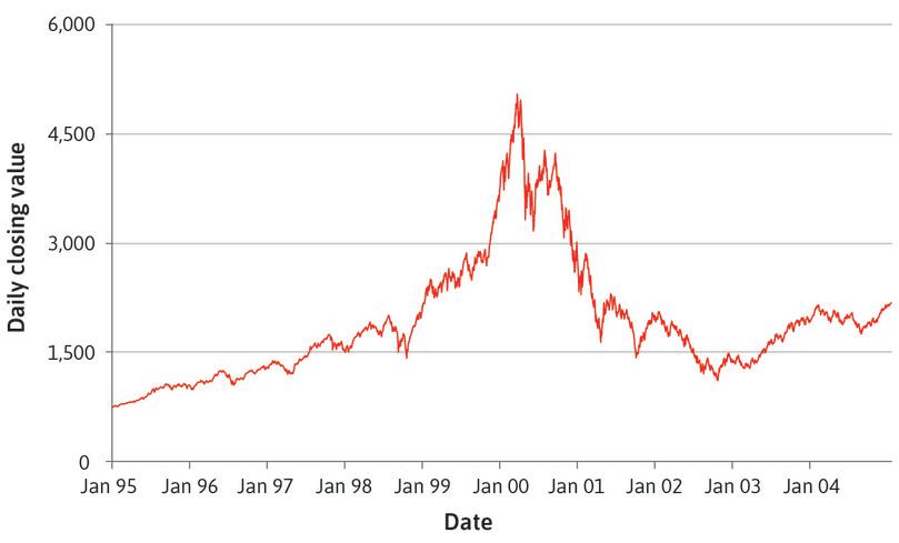
But share prices are not only volatile hour-by-hour and day-by-day. They can also display large swings, often referred to as bubbles. Figure 11.14 shows the value of the Nasdaq Composite Index between 1995 and 2004. This index is an average of prices for a set of stocks, with companies weighted in proportion to their market capitalization. The Nasdaq Composite Index at this time included many fast-growing and hard-to-value companies in technology sectors.
Yahoo Finance, accessed 14 January 2014.
The index began the period at less than 750, and rose in five years to more than 5,000 with a remarkable annualized rate of return of around 45%. It then lost two-thirds of its value in less than a year, and eventually bottomed out at around 1,100, almost 80% below its peak. The episode has come to be called the tech bubble.
Information, uncertainty, and beliefs
The term bubble refers to a sustained and significant departure of the price of any asset (financial or otherwise) from its fundamental value.
Sometimes, new information about the fundamental value of an asset is quickly and reliably expressed in markets. Changes in beliefs about a firm’s future earnings growth result in virtually instantaneous adjustments in its share price. Both good and bad news about patents or lawsuits, the illness or departure of important personnel, earnings surprises, or mergers and acquisitions can all result in active trading—and swift price movements.
Because stock price movements often reflect important information about the financial health of a firm, traders who lack this information can try to deduce it from price movements. Using Hayek’s language, changes in prices are messages containing information. If markets are to work well, traders must respond to these messages. But when they interpret a price increase as a sign of further price increases (momentum trading strategies) the result can be self-reinforcing cycles of price increases, resulting in asset price bubbles followed by sudden price declines, called crashes.
- momentum trading
- Share trading strategy based on the idea that new information is not incorporated into prices instantly, so that prices exhibit positive correlation over short periods.
Three distinctive and related features of markets may give rise to bubbles:
- Resale value: The demand for the asset arises both from the benefit to its owner (for example, the flow of dividends from a stock, or the enjoyment of having a painting by a well-known artist in your living room) and because it offers the opportunity for speculation on a change in its price. Similarly, a landlord may buy a house both for the rental income and also to create a capital gain by holding the asset for a period of time and then selling it. People’s beliefs about what will happen to asset prices differ, and change as they receive new information or believe others are responding to new information.
- Ease of trading: In financial markets, the ease of trading means that you can switch between being a buyer and being a seller if you change your mind about whether you think the price will rise or fall. Switching between buying and selling is not possible in markets for ordinary goods and services, where sellers are firms with specialized capital goods and skilled workers, and buyers are other types of firms, or households.
- Ease of borrowing to finance purchases: If market participants can borrow to increase their demand for an asset that they believe will increase in price, this allows an upward movement of prices to continue, creating the possibility of a bubble and subsequent crash.
When economists disagree Do bubbles exist?
The price movements in Figure 11.14 (and Figure 11.20 in the next section), give the impression that asset prices can swing wildly, bearing little relation to the stream of income that might reasonably be expected from holding them.
But do bubbles really exist, or are they an illusion based only on hindsight? In other words, is it possible to know that a market is experiencing a bubble before it crashes? Perhaps surprisingly, some prominent economists working with financial market data disagree on this question. They include Eugene Fama and Robert Shiller, two of the three recipients of the 2013 Nobel Prize.
Fama denies that the term ‘bubble’ has any useful meaning at all:5
These words have become popular. I don’t think they have any meaning … It’s easy to say prices went down, it must have been a bubble, after the fact. I think most bubbles are twenty-twenty hindsight. Now after the fact you always find people who said before the fact that prices are too high. People are always saying that prices are too high. When they turn out to be right, we anoint them. When they turn out to be wrong, we ignore them. They are typically right and wrong about half the time.
This is an expression of what economists call the efficient market hypothesis, which claims that all generally available information about fundamental values is incorporated into prices virtually instantaneously.6 Robert Lucas—another Nobel laureate, firmly in Fama’s camp—explained the logic of this argument in 2009, in the middle of the financial crisis:7
One thing we are not going to have, now or ever, is a set of models that forecasts sudden falls in the value of financial assets, like the declines that followed the failure of Lehman Brothers in September. This is nothing new. It has been known for more than 40 years and is one of the main implications of Eugene Fama’s efficient-market hypothesis … If an economist had a formula that could reliably forecast crises a week in advance, say, then that formula would become part of generally available information and prices would fall a week earlier.
Responding to Lucas, Markus Brunnermeier explains why this argument is not watertight:8
Of course, as Bob Lucas points out, when it is commonly known among all investors that a bubble will burst next week, then they will prick it already today. However, in practice each individual investor does not know when other investors will start trading against the bubble. This uncertainty makes each individual investor nervous about whether he can be out of (or short) the market sufficiently long until the bubble finally bursts. Consequently, each investor is reluctant to lean against the wind. Indeed, investors may in fact prefer to ride a bubble for a long time such that price corrections only occur after a long delay, and often abruptly. Empirical research on stock price predictability supports this view. Furthermore, since funding frictions limit arbitrage activity, the fact that you can’t make money does not imply that the ‘price is right’.
This way of thinking suggests a radically different approach for the future financial architecture. Central banks and financial regulators have to be vigilant and look out for bubbles, and should help investors to synchronize their effort to lean against asset price bubbles. As the current episode has shown, it is not sufficient to clean up after the bubble bursts, but essential to lean against the formation of the bubble in the first place.
Shiller has argued that relatively simple and publicly observable statistics, such as the ratio of stock prices to earnings per share, can be used to identify bubbles as they form. Leaning against the wind by buying assets that are cheap based on this criterion, and selling those that are dear, can result in losses in the short run, but long-term gains that, in Shiller’s view, exceed the returns to be made by simply investing in a diversified basket of securities with similar risk attributes.
In collaboration with Barclays Bank, Shiller has launched a product called an exchange-traded note (ETN) that can be used to invest in accordance with his theory. This asset is linked to the value of the cyclically adjusted price-to-earnings (CAPE) ratio, which Shiller believes is predictive of future prices over long periods. So this is one economist who has put his money where his mouth is: you can follow the fluctuation of Shiller’s index on Barclays Bank’s website.9
So there are two quite different interpretations of the ‘tech bubble’ episode in Figure 11.14:
- Fama’s view: Asset prices throughout the episode were based on the best information available at the time and fluctuated because information about the prospects of the companies was changing sharply. In John Cassidy’s 2010 interview with Fama in The New Yorker, he describes many of the arguments for the existence of bubbles as ‘entirely sloppy’.10
- Shiller’s view: Prices in the late 1990s had been driven up simply by expectations that the price would still rise further. He called this ‘irrational exuberance’ among investors. The first chapter of his book Irrational Exuberance explains the idea.11
- irrational exuberance
- A process by which assets become overvalued. The expression was first used by Alan Greenspan, then chairman of the US Federal Reserve Board, in 1996. It was popularized as an economic concept by the economist Robert Shiller.
Exercise 11.6 Markets for gems
A New York Times article, describes how the worldwide markets for opals, sapphires, and emeralds are affected by discoveries of new sources of gems.
- Explain, using supply and demand analysis, why Australian dealers were unhappy about the discovery of opals in Ethiopia.
- What determines the willingness to pay for gems? Why do Madagascan sapphires command lower prices than Asian ones?
- Explain why the reputation of gems from particular sources might matter to a consumer. Shouldn’t you judge how much you are willing to pay for a stone by how much you like it yourself?
- Do you think that the high reputation of gems from particular origins necessarily reflects true differences in quality?
- Could we see bubbles in the markets for gems?
Question 11.6 Choose the correct answer(s)
Which of the following statements about bubbles is correct?
- A bubble occurs when the market price deviates in a sustained and significant way from the fundamental value.
- Bubbles are more likely in these circumstances.
- Momentum traders buy or sell according to whether prices are rising or falling, rather than fundamental values, so can contribute to the formation of a bubble.
- A bubble could occur in a market for any asset that can be re-sold, for example the housing market.
11.8 Modelling bubbles and crashes
We have seen that bubbles could occur in markets for financial assets because demand depends, in part, on expectations about the prices at which they may be resold in future. This argument might also apply to durable goods—such as houses, paintings, and ‘collectibles’ like vintage cars or stamps. Can we apply our model of price-taking buyers and sellers to such markets?
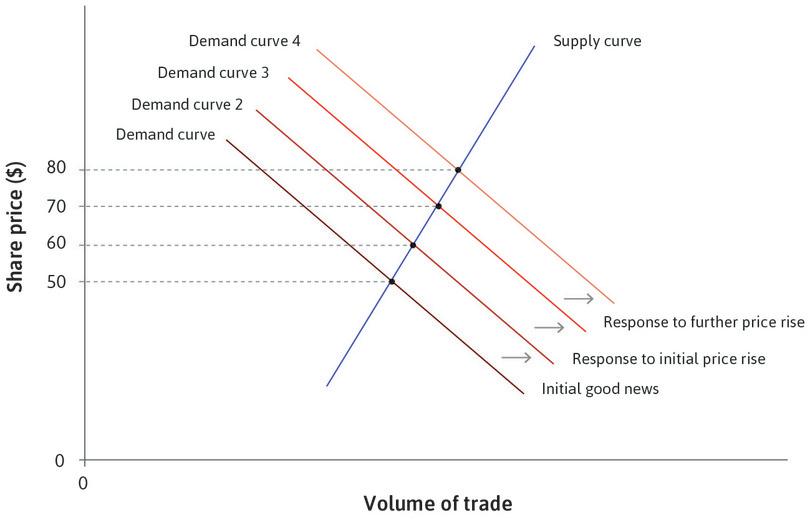
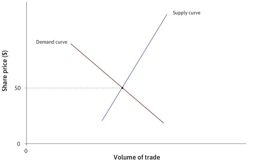
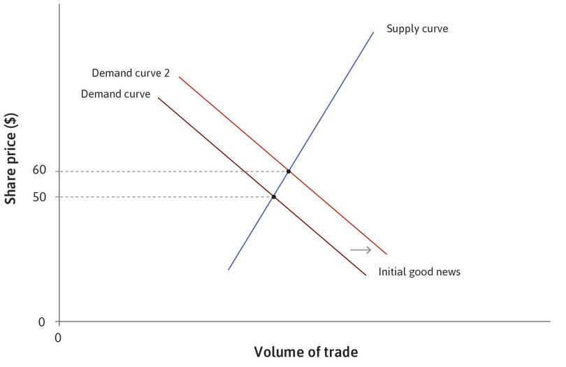
Figure 11.15 illustrates the supply and demand for shares in a (so far) hypothetical firm called the Flying Car Corporation (FCC). Initially the share price is $50 on the lowest demand curve. When potential traders and investors receive good news about expected future profitability, the demand curve shifts to the right, and the price increases to $60 (for simplicity, we assume that the supply curve doesn’t move).
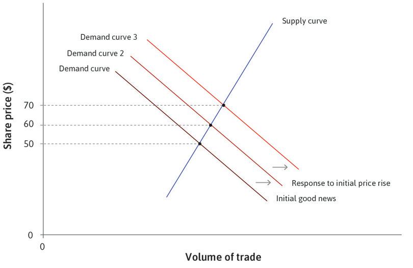
Initially the exogenous rise in demand has the same effect as in the markets for bread and hats. Follow the steps in Figure 11.15 to see what happens next.
- positive feedback (process)
- A process whereby some initial change sets in motion a process that magnifies the initial change. See also: negative feedback (process).
The sequence of events in Figure 11.15 can happen if individuals interpret a price rise to mean that other people have received news that they hadn’t heard themselves, and adjust their own expectations upwards. Or they may think there is an opportunity for speculation: to buy the stock now and sell to other buyers at a profit later. Either way, the initial increase in demand creates a positive feedback, leading to further increases in demand.
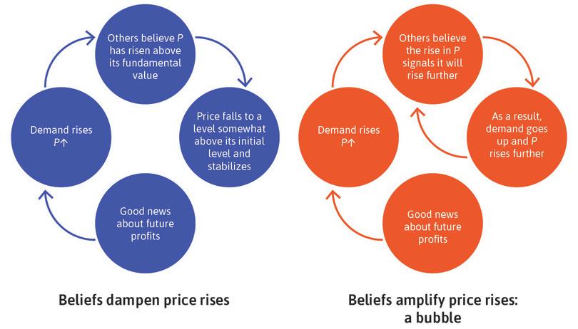
This does not happen in the bread market. People do not respond to a rise in bread price by buying more bread and filling their freezer. To model markets for assets like shares, paintings, or houses, we need to allow for the additional effects of beliefs about future prices. Figure 11.16 contrasts two alternative scenarios following an exogenous shock of good news about future profits of FCC that raises the price from $50 to $60 as in Figure 11.15.
In the left-hand panel, beliefs dampen price rises: some market participants respond to the initial price rise with scepticism about whether the fundamental value of FCC is really $60, so they sell shares, taking a profit from the higher price. This behaviour reduces the price and it falls to a value somewhat above its initial level, where it stabilizes. The news has been incorporated into a price between $50 and $60, reflecting the aggregate of beliefs in the market about the new fundamental value of FCC.
By contrast, in the right panel beliefs amplify price rises. When demand rises, others believe that the initial rise in price signals a further rise in future. These beliefs produce an increase in the demand for FCC shares. Other traders see that those who bought more shares in FCC benefited as its price rose and so they follow suit. A self-reinforcing cycle of higher prices and rising demand takes hold.
- stable equilibrium
- An equilibrium in which there is a tendency for the equilibrium to be restored after it is disturbed by a small shock.
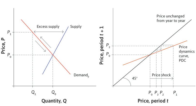
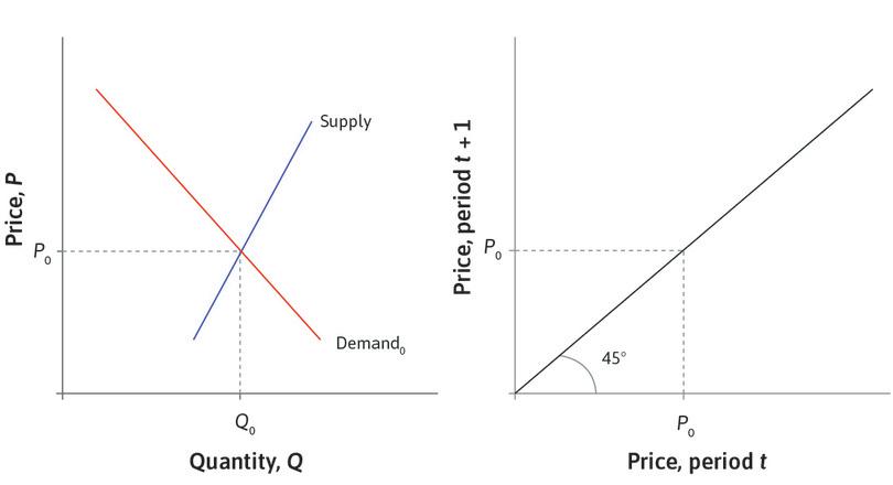
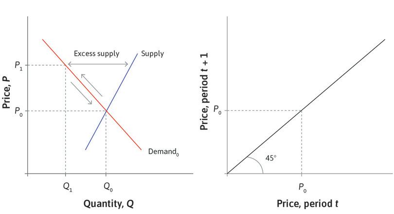
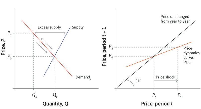
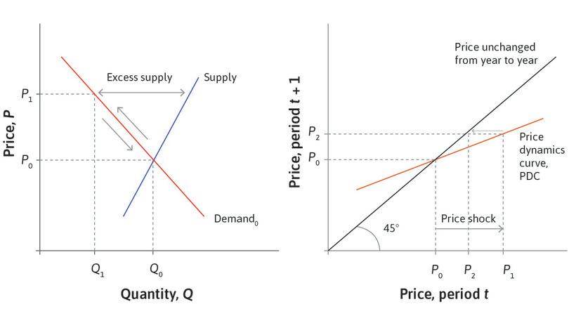
If beliefs dampen price changes and restore the market to equilibrium after a price shock, we say that the equilibrium is stable. Figure 11.17 shows how we can model the process of price adjustment in the case of a stable equilibrium. The left-hand panel shows supply and demand curves for FCC shares, with an equilibrium price P₀ corresponding to their fundamental value. The right-hand panel shows the relationship between prices in successive periods of time, called the price dynamics curve (PDC). If Pt, the price in period t, is equal to P₀, then the price in the next period, Pt+1, will be the same, because at the equilibrium there is no tendency for change. But if the current price Pt is not at the equilibrium, the PDC shows what the price will be in the next period. Follow the steps in Figure 11.7 to see how, with a PDC like the one shown here, the market will return to equilibrium after a shock.
In Figure 11.17, the PDC is flatter than the 45° line, so when the price is above the equilibrium, it will adjust downwards again until equilibrium is restored. This PDC represents the case in which beliefs about the fundamental value of the asset dominate any tendency to interpret the price rise as a signal of further price rises.
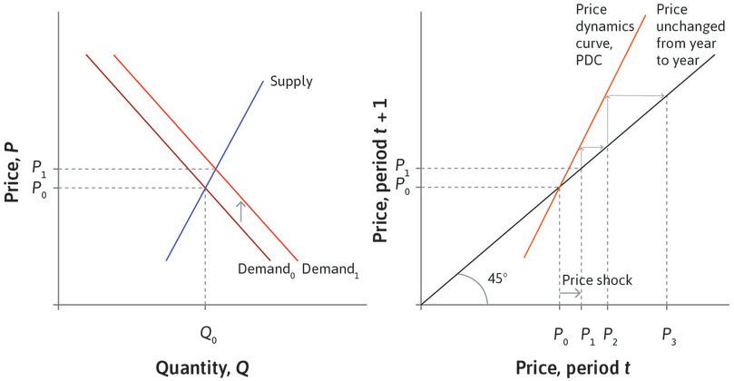
Let’s now suppose that following the initial increase in the share price P₁, demand increases: shares in FCC are now seen as a better investment. Even if everyone knows that the fundamental value of the shares is still P₀, some people believe that the price will continue to rise for some time. If the conviction takes hold that the price will increase further, then owning more shares is a good strategy. There will be a capital gain from holding them because they can be sold later for more than the price paid to acquire them.
- unstable equilibrium
- An equilibrium such that, if a shock disturbs the equilibrium, there is a subsequent tendency to move even further away from the equilibrium.
In this case, as shown in the left-hand panel of Figure 11.18, the higher price shifts the demand curve to the right. In the right-hand panel, the PDC is steeper than the 45° line. This tells us that the price next period is further from the equilibrium at P₀ than the price this period. This PDC represents the case of an unstable equilibrium.
In the next period the price rises again. In a self-reinforcing bubble, this process can continue indefinitely—at least until something happens to change the expectation of continuously rising prices (and of a growing deviation of the price from its fundamental value).
Instability caused by self-reinforcing price expectations can only happen in markets for goods that can be resold, like financial assets or durable goods. There is no point buying more vegetables, fish, or fashion items in the hope of making a capital gain on them, because the fish and vegetables will rot, and fashions will change. However, in the markets for tulip bulbs in the seventeenth century, office space in Tokyo in the late 1980s, and houses in Las Vegas in the 2000s (see Exercise 11.10), people continued buying as prices rose, accelerating prices further, because they expected to benefit by reselling the asset.
In Unit 17 we will use a model with a price dynamics curve to look at the role of the housing market in the financial crisis of 2008. In Unit 20, a similar model helps explain how humans interact with the natural environment and why in some situations we observe both stabilizing processes and vicious circles of runaway environmental collapse.
Leibniz: Price bubbles
How do bubbles come to an end?
A bubble bursts when some participants in the market perceive a danger that the price will fall. Then would-be buyers hold back, and those who hold the assets will try to get rid of them. The process in Figure 11.15 is reversed. Figure 11.19 uses the supply and demand model to illustrate what happens. At the top of the bubble the shares trade at $80. Both the supply and demand curves shift when the bubble bursts, and the price collapses from $80 to $54—leaving those who owned shares when the price was $80 with large losses.
If the price of an asset has been driven up solely by beliefs about future price rises, there should be opportunities for those who are well informed about the value to profit from their superior information. So if the rise in the Nasdaq index in Figure 11.14 was indeed a bubble, why did those who identified it as a bubble fail to profit by placing gigantic bets on a major price decline?
- short selling
- The sale of an asset borrowed by the seller, with the intention of buying it back at a lower price. This strategy is adopted by investors expecting the value of an asset to decrease. Also known as: shorting.
As it happens, many large investors did ‘lean against the wind’ by placing bets on the bubble bursting, including some well-known fund managers on Wall Street. They did so by selling short (shorting): borrowing shares at the current high price and immediately selling them, with the intention of buying them back cheaply (to return to the owner) after the price crashed. But this is an extremely risky strategy, since it requires accuracy in timing the crash—if prices continue to rise, the losses can become unsustainable. You may be right about the bubble but if you get the timing wrong, then when you are due to buy the shares and return them to the owner, the price is higher than it was when you sold them. You will make a loss and may not be able to repay your loan.
Indeed, many of those buying an asset may also be convinced of an eventual crash, but hoping to exit the market before it happens. This was the case during the tech bubble when Stanley Druckenmiller, manager of the Quantum Fund with assets of $8 billion, held shares in technology companies that he knew were overvalued. After prices collapsed and inflicted significant losses on the fund, he used a baseball metaphor to describe his error. ‘We thought it was the eighth inning, and it was the ninth,’ he explained, ‘I overplayed my hand.’
Exercise 11.7 What is the fundamental value of a Bitcoin?
A bubble may have occurred in the market for the virtual currency called Bitcoin. Bitcoin was introduced by a group of software developers in 2009. Where it is accepted, it can be transferred from one person to another as payment for goods and services.
Unlike other currencies it is not controlled by a single entity such as a central bank. Instead it is ‘mined’ by individuals who lend their computing power to verify and record Bitcoin transactions in the public ledger. At the start of 2013, a Bitcoin could be purchased for about $13. On 4 December 2013 it was trading at $1,147. It then lost more than half its value in two weeks. These and subsequent price swings are shown in Figure 11.20.
Coindesk.com. 2015. Bitcoin News, Prices, Charts, Guides & Analysis and Bitcoincharts. Both accessed August 2016.
Use the models in this section, and the arguments for and against the existence of bubbles, to provide an account of the data in Figure 11.20.
Exercise 11.8 The big ten asset price bubbles of the last 400 years
According to Charles Kindleberger, an economic historian, asset price bubbles have occurred across a wide variety of countries and time periods. The bubbles of the last 100 years have predominantly been focused on real estate, stocks, and foreign investment.12
- 1636: The Dutch tulip bubble
- 1720: The South Sea Company
- 1720: The Mississippi Scheme
- 1927–29: The 1920s stock price bubble
- 1970s: The surge in loans to Mexico and other developing economies
- 1985–89: The Japanese bubble in real estate and stocks
- 1985–89: The bubble in real estate and stocks in Finland, Norway and Sweden
- 1990s: The bubble in real estate and stocks in Thailand, Malaysia, Indonesia and several other Asian countries between 1992 and 1997, and the surge in foreign investment in Mexico 1990–99
- 1995–2000: The bubble in over-the-counter stocks in the US
- 2002–07: The bubble in real estate in the US, Britain, Spain, Ireland, and Iceland
Pick one of these asset price bubbles, find out more about it, and then:
- Tell the story of this bubble using the models in this section.
- Explain the relevance to your story, if any, of the arguments in the ‘Do bubbles exist?’ box in Section 11.7 about the existence of bubbles.
Question 11.7 Choose the correct answer(s)
Which of the following statements about asset prices are correct?
- When beliefs amplify a price rise, the price moves further away from the fundamental value, causing a bubble.
- Positive feedback is when an initial price change sets in motion a process that magnifies the initial change, so the market moves further away from equilibrium.
- Negative feedback is when an initial price change is dampened by other market participants selling the asset, in the belief that the price is now above the fundamental value.
- If beliefs about the fundamental value dampen a price rise, the market moves back to equilibrium.
Question 11.8 Choose the correct answer(s)
Which of the following statements about short selling (shorting) is correct?
- Shorting allows a trader to benefit by selling borrowed shares while the price is high, and buying them back (to return to the owner) when the price has fallen.
- Shorting involves selling shares that you have borrowed.
- Once you have sold the shares at a certain price, there is no limit to the amount of loss you can incur, as the price can keep rising.
- Shorting works only if your timing is correct (just as the bubble bursts). Otherwise the strategy can result in a large loss.
11.9 Non-clearing markets: Rationing, queuing, and secondary markets
Tickets for Beyoncé’s 2013 world tour sold out in 15 minutes for the Auckland show in New Zealand, in 12 minutes for three UK venues, and in less than a minute for Washington DC in the US. When American singer Billy Joel announced a surprise concert in his native Long Island, New York in October 2013, all available tickets were snapped up in minutes. In both cases it’s safe to say that there were many disappointed buyers who would have paid well above the ticket price. At the price chosen by the concert organizers, demand exceeded supply.
We see excess demand for tickets for sporting events, too. The London organizing committee for the 2012 Olympic games received 22 million applications for 7 million tickets. Figure 11.21 is a stylized representation of the situation for one Olympic event.
The number of available tickets, 40,000, is fixed by the capacity of the stadium. The ticket price at which supply and demand are equal is £225. The organizing committee do not choose this price, but a lower price of £100; at this price 70,000 tickets are demanded. There is excess demand of 30,000 tickets.
Some of those who obtain tickets for a popular event may be tempted to sell them rather than use them. In Figure 11.21, anyone who buys a ticket for £100 with the intention of reselling could sell it for at least £225, receiving a rent of £125 (compared with the next best alternative of not buying a ticket).
The potential for rents may create a parallel or secondary market. In the case of tickets for concerts and sporting events, part of the initial demand comes from scalpers: people who plan to resell at a profit. Tickets appear almost instantly on peer-to-peer trading platforms such as StubHub or Ticketmaster, listed at prices that may be multiples of what was originally paid. In the last few days of the 2014 Winter Olympics in Sochi, tickets for the Olympic Park with a face value of 200 roubles were sold outside the Park for up to 4,000 roubles.
Prices in the secondary market equate demand and supply, and allocations are accordingly made to those with the greatest willingness to pay. The assumption that this market-clearing price will be much higher than the listed price is responsible, in part, for the initial frenzied demand for tickets. Nevertheless, some individuals who buy at the lower prices hold on to their tickets, and attend an event that they would otherwise be unable to afford.
Event organizers may try to prevent scalping. In Sochi, the security officers were supposed to intervene. But prevention is increasingly difficult, as online sales provide new opportunities for scalping on a large scale using ‘ticket-bots’: software that automatically buys tickets within moments of their release. The New York Times estimated that scalpers made $15.5 million from just 100 performances of the Broadway musical Hamilton in the summer of 2016.
- rationed goods
- Goods that are allocated to buyers by a process other than price (such as queueing, or a lottery).
In the case of the London Olympics, the organizing committee set the price, and the tickets were allocated by lottery. This is an example of goods being rationed rather than allocated by price. The organizers could have chosen a much higher price (£225 for the event in Figure 11.21), which would have cleared the market. But that would have meant that people willing to pay less than £225 would not have seen the event. By allocating the tickets through a lottery, some people with a lesser willingness to pay (perhaps because they had limited incomes) would also get to see the Games.
There was much public debate about the process, and some anger, but IOC President Jacques Rogge defended it as ‘open, transparent and fair’.
There are other cases where the producer of a good chooses to operate with persistent excess demand. The New York restaurant Momofuku Ko offers a 16-course tasting menu at lunch for $175, and has just 12 seats. Online reservations may be made one week in advance, open at 10 a.m. daily, and typically sell out in three seconds. In 2008, the proprietor David Chang sold a reservation at a charity auction for $2,870. Even taking into account the willingness of individuals to pay more for an item when the proceeds go to charity, this suggests substantial excess demand for reservations—but he has not raised the price.
Exercise 11.9 IOC policy
- Do you think the IOC policy of using a lottery is fair?
- Is it Pareto efficient? Explain why or why not.
- Using the criteria of fairness and Pareto efficiency, how would you judge the widely criticized practice of ‘scalping’ tickets.
- Can you think of any other arguments for or against scalping?
Exercise 11.10 The price of a ticket
Explain why the seller of a good in fixed supply (such as concert tickets or restaurant reservations) might set a price that the seller knows to be too low to clear the market.
Question 11.9 Choose the correct answer(s)
Figure 11.21 is a stylized representation of the market for an event at the 2012 London Olympic Games. 40,000 tickets were allocated by lottery, at £100 each.
Assume that buyers could resell their tickets in the secondary market. Which of the following statements is correct?
- The market would have cleared at £225 for the supply of 40,000 tickets.
- 70,000 people wanted tickets, but only 40,000 were allocated, randomly.
- In the secondary market the ticket could be sold at £225, making the economic rent earned £125.
- With supply limited to 40,000, selling them all at £225 would have increased the organizers’ profit. But they preferred to set a price that was affordable for more people.
11.10 Markets with controlled prices
In December 2013, on an unusually cold and snowy Saturday in New York City, demand for taxi services rose appreciably. The familiar metered yellow and green cabs, which operate at a fixed rate (subject to minor adjustments for peak and night-time hours), were hard to find. Those looking for taxis were accordingly rationed, or faced long waiting times.
But there was an alternative available—another example of a secondary market: the on-demand, app-based taxi service called Uber, which by March 2017 would be operating in 81 countries. This recent entrant in the local transportation market uses a secret algorithm that responds rapidly to changing demand and supply conditions.
Standard cab fares do not change with the weather, but Uber’s prices can change substantially. On this December night, Uber’s surge-pricing algorithm resulted in fares that were more than seven times Uber’s standard rate. This spike in pricing choked off some demand and also led to some increased supply, as drivers who would have clocked off remained on the road and were joined by others.
City authorities often regulate taxi fares as part of their transport policy, for example to maintain safety standards, and minimize congestion. In some countries, local or national government also controls housing rents. Sometimes this is to protect tenants, who may have little bargaining power in their relationships with landlords, or sometimes because urban rents would be too high for key groups of workers.
Figure 11.22 shows a situation in which local government might decide to control the housing rent in a city (note that here we mean rent in the everyday sense of a payment from tenant to landlord for use of the accommodation). Initially the market is in equilibrium, with 8,000 tenancies at a rent of €500—the market clears. Now suppose that there is an increase in demand for tenancies. Rents will rise, because the supply of rental housing is inelastic, at least in the short run: it would take time to build new houses, so more tenancies can only be supplied immediately if some owner-occupiers decide to become landlords and live elsewhere themselves.
- rent ceiling
- The maximum legal price a landlord can charge for a rent.
Suppose that the city authorities are concerned that this rise would be unaffordable for many families, so they impose a rent ceiling at €500. Follow the steps in Figure 11.22 to see what happens.
- short side (of a market)
- The side (either supply or demand) on which the number of desired transactions is least (for example, employers are on the short side of the labour market, because typically there are more workers seeking work than there are jobs being offered). The opposite of short side is the long side. See also: supply side, demand side.
With a controlled price of €500 there is excess demand. In general a controlled price will not clear the market, and trade will then take place on the short side of the market: that is, the quantity traded will be whichever is lower of the quantities supplied and demanded. In Figure 11.22, the price is low and suppliers are on the short side. If the price were high (above the market-clearing price), demanders would be on the short side.
When the rent is €500, the number of tenancies will be 8,000. Of the 12,000 people on the long side of the market, 8000 would pay €1,100 or more, but tenancies are not allocated to those with highest willingness to pay. Those lucky enough to obtain tenancies may be anywhere on the new demand curve above €500.
This brief economic analysis of rent controls in Paris points out the counter-productive effects: Jean Bosvieux and Oliver Waine. 2012. ‘Rent Control: A Miracle Solution to the Housing Crisis?’. Metropolitics. Updated 21 November 2012.
Richard Arnott, on the other hand, argues that economists should rethink their traditional opposition to rent control: Richard Arnott. 1995. ‘Time for Revisionism on Rent Control?’. Journal of Economic Perspectives 9 (1) (February): pp. 99–120.
The rent control policy puts more weight on maintaining a rent that is seen to be fair, and affordable by existing tenants who might otherwise be forced to move out, than it does on Pareto efficiency. The scarcity of rental accommodation gives rise to a potential economic rent: if it were legal (it usually isn’t), some tenants could sublet their accommodation, obtaining an economic rent of €600 (the difference between €1,100 and €500).
If the increase in demand proves to be permanent, the long-run solution for the city authorities may be policies that encourage house-building, shifting out the supply curve so that more tenancies are available at a reasonable rent.
Exercise 11.11 Why not raise the price?
Discuss the following statement: ‘The sharp increase in cab fares on a snowy day in New York led to severe criticism of Uber on social media, but a sharp increase in the price of gold has no such effect.’
Question 11.10 Choose the correct answer(s)
Figure 11.22 illustrates the rental housing market. Initially, the market clears at €500 with 8,000 tenancies. Then, there is an outward shift in the demand curve, as shown in the diagram. In response, the city authority imposes a rent ceiling of €500 and prohibits subletting. Based on this information, which of the following statements are correct?
- At €500, 12,000 people want tenancies, but there are only 8,000 available.
- The market would clear at €830.
- Those subletting would be able to charge a rent of €1,100 under the new demand curve, obtaining economic rent of €600.
- If enough houses were built the supply curve would shift outwards and the market would again clear at €500.
11.11 The role of economic rents
An economic rent is a payment or other benefit that someone receives that is superior to his or her next best alternative. Throughout this unit, we have seen how economic rents play a role in the changes that take place in the economy.
- In the real case of the Kerala fisherman, and the hypothetical market for hats, rent-seeking by buyers or sellers in response to a situation of excess supply or demand brought about a market-clearing equilibrium.
- In the model of the bread market, rents (economic profits) can arise in a short-run equilibrium in which the number of firms is fixed. In the long run, other bakeries enter the market in pursuit of these rents.
- In the world oil market, rents for oil producers arise from the constraints on producers and consumers that make supply and demand curves inelastic in the short-run, but in turn provide incentives for building new wells for exploration.
- In asset markets, rents arise when the price deviates from the fundamental value of the asset, providing opportunities for speculation and creating the potential for bubbles.
- In markets that do not clear because prices are controlled, excess demand gives rise to a potential economic rent, which leads (unless prevented by regulation) to the development of a clearing secondary market.
- Another example, from Unit 2, is the innovation rent obtained by early innovators, which provides the incentive to adopt a new technology.
- disequilibrium rent
- The economic rent that arises when a market is not in equilibrium, for example when there is excess demand or excess supply in a market for some good or service. In contrast, rents that arise in equilibrium are called equilibrium rents.
- equilibrium rent
- Rent in a market that is in equilibrium. Also known as: stationary or persistent rents.
In each of these examples, rents arise because of some kind of disequilibrium, or short-run constraint—we call them dynamic or disequilibrium rents. They set in motion a process—rent-seeking—that ultimately creates an equilibrium in which these kinds of rents no longer exist. In contrast, we have also seen examples of persistent or stationary rents. The main examples are shown in the table in Figure 11.23.
| Type | Description | Unit |
|---|---|---|
| Bargaining | In a bargaining situation, how much the outcome exceeds the reservation option (next best alternative) | 4.5 |
| Employment | Wages and conditions above an employee’s reservation option providing an incentive to work hard | 6.9 |
| Monopoly | Profits above economic profits made possible by limited competition | 7 |
| Government-induced | Payments above the actor’s next best alternative not competed away because of government regulation (for example rent control, intellectual property rights) | 9 |
Examples of stationary rents.
Figure 11.23 Examples of stationary rents.
In the models studied in this unit, we have seen that if markets do not clear, there are disequilibrium rents that give incentives for people to change the prices or quantities at which they transact, and so bring about market clearing. The labour market (see Unit 9) is different: it does not clear in equilibrium. Employees therefore receive a rent—the difference between the wage and their reservation option. But in this case it is a persistent or equilibrium rent: because a contract to work hard is unenforceable there is no way any buyer (the employer) or seller (the worker) can benefit by changing his or her price or quantity.
Economic rents and rent-seekers often have a bad name in economics. People disapprove because they think about rents as those arising from government-created monopolies (taxi licenses, intellectual property rights) or privately created monopolies. These rents indicate that the good or service will be sold at a price exceeding its marginal cost, and so the markets for these goods are not Pareto efficient.
But we have now seen the usefulness of some economic rents. They encourage innovation, provide incentives for employees to work hard, encourage new entrants to a market and thereby lower prices for consumers, and can bring an out-of-equilibrium market to a Pareto-efficient equilibrium.
Question 11.11 Choose the correct answer(s)
Which of the following are stationary rents?
- Innovation rent is only temporary until other firms catch up—it is a dynamic rent.
- Employers will continue to pay wages above the reservation wage, because otherwise employees would reduce their work effort.
- When competition is limited, firms will continue to produce where price is greater than marginal cost.
- This is clearly not permanent!
11.12 Conclusion
Prices are messages about the conditions in a market economy. In situations of market disequilibrium, or short-run equilibrium arising from temporary constraints, people act on price messages if they are able to do so, in pursuit of economic rents. In markets for goods this often leads in the long run to market clearing and the eventual disappearance of the rents.
Assets are purchased partly for their resale value. In markets for financial assets, supply and demand shift rapidly as traders receive new information. The price adjusts in a continuous double auction to reconcile supply and demand. Prices in asset markets send messages to traders about future prices, which can cause the price to deviate from the fundamental asset value; in this case rent-seeking may create a bubble or a crash.
Sometimes suppliers or regulators choose to override price messages, leading to excess supply or demand, for example for concert tickets, taxi cabs, or housing tenancies. Economic rents can then persist—unless a secondary market is allowed to develop.
Concepts introduced in Unit 11
Before you move on, review these definitions:
- Market equilibration through rent-seeking
- Long-run and short-run equilibria
- Fundamental value of an asset
- Continuous double auction
- Order book
- Price bubble
- Stable and unstable equilibria
- Secondary market
- Dynamic and stationary economic rents
11.13 References
- Arnott, Richard. 1995. ‘Time for Revisionism on Rent Control?’. Journal of Economic Perspectives 9 (1) (February): pp. 99–120.
- Bosvieux, Jean, and Oliver Waine. 2012. ‘Rent Control: A Miracle Solution to the Housing Crisis?’. Metropolitics. Updated 21 November 2012.
- Brunnermeier, Markus. 2009. ‘Lucas Roundtable: Mind the frictions’. The Economist. Updated 6 August 2009.
- Cassidy, John. 2010. ‘Interview with Eugene Fama’. The New Yorker. Updated 13 January 2010.
- Harford, Tim. 2012. ‘Still Think You Can Beat the Market?’. The Undercover Economist. Updated 24 November 2012.
- Hayek, Friedrich A. 1994. The Road to Serfdom. Chicago, Il: University of Chicago Press.
- Keynes, John Maynard. 1936. The General Theory of Employment, Interest and Money. London: Palgrave Macmillan.
- Kindleberger, Charles P. 2005. Manias, Panics, and Crashes: A History of Financial Crises (Wiley Investment Classics). Hoboken, NJ: Wiley, John & Sons.
- Lucas, Robert. 2009. ‘In defence of the dismal science’. The Economist. Updated 6 August 2009.
- Malkiel, Burton G. 2003. ‘The Efficient Market Hypothesis and Its Critics’. Journal of Economic Perspectives 17 (1) (March): pp. 59–82.
- Miller, R. G., and S. R. Sorrell. 2013. ‘The Future of Oil Supply’. Philosophical Transactions of the Royal Society A: Mathematical, Physical and Engineering Sciences 372 (2006) (December).
- Owen, Nick A., Oliver R. Inderwildi, and David A. King. 2010. ‘The Status of Conventional World Oil Reserves—Hype or Cause for Concern?’. Energy Policy 38 (8) (August): pp. 4743–4749.
- Shiller, Robert J. 2003. ‘From Efficient Markets Theory to Behavioral Finance’. Journal of Economic Perspectives 17 (1) (March): pp. 83–104.
- Shiller, Robert J. 2015. ‘The Stock Market in Historical Perspective’. In Irrational Exuberance. Princeton, NJ: Princeton University Press.
- The Economist. 2014. ‘Keynes and Hayek: Prophets for Today’. Updated 14 March 2014.
-
Friedrich A. Hayek. 1994. The Road to Serfdom. Chicago, Il: University of Chicago Press. ↩
-
‘Keynes and Hayek: Prophets for Today’. The Economist. Updated 14 March 2014. ↩
-
R. G. Miller and S. R. Sorrell. 2013. ‘The Future of Oil Supply’. Philosophical Transactions of the Royal Society A: Mathematical, Physical and Engineering Sciences 372 (2006) (December). ↩
-
Nick A. Owen, Oliver R. Inderwildi, and David A. King. 2010. ‘The status of conventional world oil Reserves—Hype or cause for concern?’ Energy Policy 38 (8) (August): pp. 4743–4749. ↩
-
Eugene Fama, quoted in ‘Interview with Eugene Fama’, The New Yorker. (2010). ↩
-
Tim Harford. 2012. ‘Still Think You Can Beat the Market?’. The Undercover Economist. Updated 24 November 2012. ↩
-
If the efficient market hypothesis is accurate, how could the 2008 financial crisis happen? Robert Lucas on Fama’s efficient market hypothesis: Robert Lucas. 2009. ‘In Defence of the Dismal Science’. The Economist. Updated 6 August 2009. ↩
-
Brunnermeier argues Lucas was right to emphasize that financial market frictions are a counter-argument to the efficient market hypothesis: Markus Brunnermeier. 2009. ‘Lucas Roundtable: Mind the Frictions’. The Economist. Updated 6 August 2009.
Robert J. Shiller. 2003. ‘From Efficient Markets Theory to Behavioral Finance’. Journal of Economic Perspectives 17 (1) (March): pp. 83–104.
Burton G. Malkiel. 2003. ‘The Efficient Market Hypothesis and Its Critics’. Journal of Economic Perspectives 17 (1) (March): pp. 59–82. ↩
-
The classic examination of bubbles was made by John Maynard Keynes in Chapter 12 of his General Theory. John Maynard Keynes. 1936. The General Theory of Employment, Interest and Money. London: Palgrave Macmillan. ↩
-
John Cassidy. 2010. ‘Interview with Eugene Fama’. The New Yorker. Updated 13 January 2010. ↩
-
Robert J. Shiller. 2015. Irrational Exuberance, Chapter 1. Princeton, NJ: Princeton University Press. ↩
-
Charles P. Kindleberger. 2005. Manias, Panics, and Crashes: A History of Financial Crises (Wiley Investment Classics). Hoboken, NJ: Wiley, John & Sons. ↩
