Leibniz

6.6.1 The worker’s best response function

We have represented the interaction between a worker and an employer as a game in which the employer chooses the wage, and the worker responds by choosing how hard to work. In this Leibniz we describe the mathematical properties of the worker’s response.

The worker, Maria, cares about two things: her income, and not having to work too hard. But work is worth more to her than her next best option, which is unemployment—she earns an employment rent. While employed, she can choose how hard to work. Her level of effort, $e$, is the proportion of each hour she spends working. If she puts in too little effort, she risks being fired, and losing her employment rent. The size of the employment rent depends, in particular, on the wage chosen by her employer. For each level of the wage, $w$, she chooses the level of effort, $e$, that is her best response to the situation she faces. Her best response curve is a function that tells us the level of effort chosen at each level of the wage:

$$e = E(w)$$

To model Maria’s decision fully, we could start from her utility function, and solve her utility maximization problem to find her best response to each wage. But in this unit we are focusing on the interaction between Maria and her employer. So we skip this step and simply describe what shape we would expect her best response function to have (so that we can draw it) by thinking about how she makes her decision.

The shape of the best response function

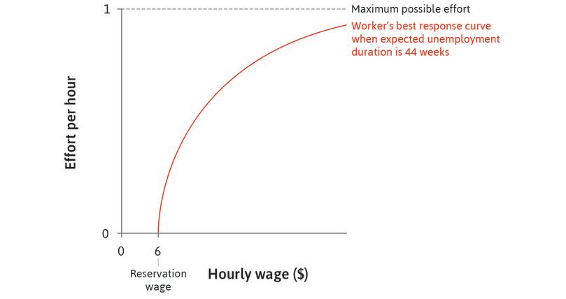
The best response function we drew in the text has the shape shown in Figure 1. The wage chosen by the employer is on the horizontal axis, and the corresponding level of effort chosen by Maria is on the vertical axis.

Why would we expect the function to look like this? First, if the wage is equal to the reservation wage, her employment rent is zero, so she will exert no effort. Hence the function crosses the horizontal axis at the reservation wage. Secondly, Maria works harder if she is paid more. This happens because, as the wage increases, so does the employment rent. So she chooses higher effort, to reduce the risk of being fired and losing the rent. Thus the curve slopes upward. In other words, $E(w)$ is an increasing function of $w$:

$$E'(w)\gt0$$

The third property you can see in Figure 1 is that the slope of the function $E(w)$ falls as $w$ increases. This feature arises if, as we would expect, the marginal cost (or disutility) of effort increases as effort increases. The higher the wage, the higher Maria’s effort—but the more difficult it is for her to increase her effort further if the wage increases a little more. This means that the function $E(w)$ is concave, and so:

$$E''(w)\lt0$$

Other influences on the best response function

The employment rent, which gives Maria the incentive to work hard, does not only depend on the wage. Section 6.5 of the text discussed the components of the employment rent in detail. The rent per hour consists of the difference between the wage and Maria’s reservation income (such as unemployment benefits from the government, or the value of the help from her family), less the disutility of effort. The total rent is the rent per hour multiplied by the expected duration of unemployment (before she finds another job).

Maria’s choice of effort will also depend on how closely she is monitored by her employer. The higher the probability that she will be caught during any minute spent checking Facebook, the greater the incentive to work hard.

These additional factors affecting effort determine the position of the best response curve in the $w-e$-plane and are known as parameters of the best response function $E$. Changes in the values of the parameters shift the best response curve. For example, an increase in the unemployment duration will increase the level of effort at each wage, shifting the curve upward, and an increase in unemployment benefit would shift it downward.

We may describe the effects of non-wage factors by treating them as additional variables. Maria’s best response function could be written as a function of five variables rather than one:

$$e = E(w,\ a,\ p,\ b,\ d)$$

where

• $e$ and $w$ again stand for effort and wage respectively

• $a$ is a measure of the disutility of effort, a feature of Maria’s utility function

• $p$ is the probability of getting caught when she is not working

• $b$ is her unemployment benefit

• $d$ stands for the duration of unemployment

For given values of the additional variables $a$, $p$, $b$ and $d$, the relationship between $e$ and $w$ has the shape shown in Figure 1—$E$ is an increasing and concave function of $w$. The only difference is that we express this using partial derivatives:

$$\frac{\partial E}{\partial w} \gt0, \, \frac{\partial^2 E}{\partial w^2} \lt0$$

The effects of the other variables can also be expressed as partial derivatives. From the discussion above we can see that:

$$\frac{\partial E}{\partial a} \lt 0, \, \frac{\partial E}{\partial p} \gt 0, \, \frac{\partial E}{\partial b} \lt 0, \, \frac{\partial E}{\partial d} \gt 0.$$

Thus Maria’s effort is a decreasing function of disutility of effort and unemployment benefit, and an increasing function of the probability of being caught shirking and the duration of unemployment.

Read more: Section 14.1 of Malcolm Pemberton and Nicholas Rau. 2015. Mathematics for economists: An introductory textbook, 4th ed. Manchester: Manchester University Press.