Leibniz

7.5.1 The profit-maximizing price

To maximize its profit, Beautiful Cars chooses a point on its demand curve where its isoprofit curve is tangent to the demand curve. We have seen this diagrammatically, and in this Leibniz we prove that the tangency point is optimal by solving the profit-maximization problem mathematically.

The demand curve for Beautiful Cars slopes downward. When choosing a price, the managers of the firm know that the more cars they produce, the lower the price they will need to set in order to sell them. In the text, we drew the demand curve as a downward-sloping straight line, but in reality it is unlikely to be straight. Here we express it more generally as a function. The maximum price $P$ at which $Q$ cars can be sold is given by:

$$P=f(Q)$$

where $f$ is a strictly decreasing function ($f'(Q)\lt0$). When we write the demand relationship like this, with price as a function of quantity, we call $f$ the inverse demand function. When it is written the other way around, with quantity in terms of price, the function is called the demand function.

Beautiful Cars’ profit, $\Pi$, is equal to its total revenue minus its total cost:

$$\Pi = PQ - C(Q)$$

The company wishes to set price and quantity so as to maximize its profit, subject to the constraint that the price is one that buyers are willing to pay. Its problem is therefore to:

$$\begin{align*}\text{choose }Q \text{ and } P \text{ to maximize }PQ - C(Q) \text{ subject to }P = f(Q)\end{align*}$$

The simplest way to solve this optimization problem is by the method of substitution. We use the constraint to substitute for $P$, giving profit as a function of $Q$ alone:

$$\Pi= Qf(Q) - C(Q)$$

To find the value of $Q$ that maximizes this function, we differentiate with respect to $Q$ (using the product differentiation rule, $\dfrac{d}{dQ}(Qf(Q)) =$ $f(Q) + Qf'(Q)$):

$$\frac{d\Pi}{dQ} = f(Q) + Qf'(Q) - C'(Q)$$

The first-order condition for optimization is $d\Pi/dQ = 0$, which may be rearranged as follows:

$$f'(Q)= \frac{C'(Q) - f(Q)}{Q}$$

The profit-maximizing quantity, $Q^*$, satisfies this equation. If we knew the specific form of the functions $f(Q)$ and $C(Q)$, we could try to solve the equation to find $Q^*$ explicitly. The profit-maximizing price could then be calculated as $P^*=f(Q^*)$.

But without knowing the functions, we can still interpret the first-order condition. We know that the optimal value of $Q$ is on the demand curve, so $f(Q) = P$, and that $C'(Q)$ is marginal cost (MC). So the first-order condition can be written:

$$f'(Q)= \frac{C'(Q) - f(Q)}{Q}$$

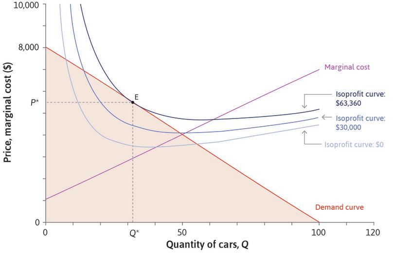
The left-hand side of this equation is the slope of the demand curve. We showed in Leibniz 7.4.1 that the right-hand side is the slope of the isoprofit curve. Thus the first-order condition tells us precisely that the profit-maximizing choice lies at a point of tangency between the demand and isoprofit curves. For Beautiful Cars, this is point E in Figure 7.11, reproduced below as Figure 1.

Notice that the left-hand side of the first-order condition, $f'(Q)$, is negative, so the right-hand side must also be negative. The profit-maximizing point lies on the downward-sloping part of an isoprofit curve, where price exceeds marginal cost.

Read more: Sections 6.4, 7.4, and 8.1 of Malcolm Pemberton and Nicholas Rau. 2015. Mathematics for economists: An introductory textbook, 4th ed. Manchester: Manchester University Press.