Leibniz

7.3.1 Average and marginal cost functions

The total costs of production for a manufacturing firm such as Beautiful Cars include the rent on the factory, the lease on equipment and machinery, the price of raw materials (including utilities), and the wages of all its employees. The cost function, $C(Q)$, describes how the firm’s total costs vary with its output—the number of cars, $Q$, that it produces. In this Leibniz we show how the firm’s average and marginal cost functions are related to $C(Q)$.

In general, total costs will increase with the quantity of output produced. In what follows, we treat $Q$ as a continuous variable, a common and useful approximation when dealing with large numbers. It then makes sense to assume that the function $C$ is differentiable, and describe the fact that it is an increasing function by the inequality:

$$C'(Q)\gt0$$

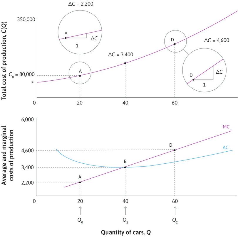
The graph of the function $C$ is shown in the upper panel of Figure 7.7 of the text, reproduced below as Figure 1. Note that $C(0)=F\gt0$; even if no cars are produced the firm incurs some costs, $F$, referred to as fixed costs. In the diagram, $C$ is an increasing function and it is also convex: the slope of the curve increases as $Q$ increases. We shall say more about this below.

The average cost (AC) of producing Beautiful Cars is defined as the total cost divided by the number of cars produced. Thus if $Q$ cars are produced:

$$\text{AC} = \frac{C(Q)}{Q}$$

In the upper panel of Figure 1, the average cost of producing $Q$ cars is the slope of the line from the point $(Q, C(Q))$ to the origin. And you can see from the diagram that the slope varies with $Q$: the average cost AC is itself a function of $Q$. The graph of the function $AC(Q)$ is shown in the lower panel of Figure 1.

The marginal cost (MC) is the rate at which costs increase if $Q$ increases. Thus if $Q$ cars are produced:

$$\text{MC} =C'(Q)$$

You can interpret MC, as in the text, as the cost of producing one more car: but remember that this is only an approximation. Geometrically, MC is the slope of the curve $C(Q)$ shown in the upper panel of Figure 1. As mentioned earlier, this cost function has the property that the slope increases as $Q$ increases: we are assuming that for Beautiful Cars the cost of producing an additional car is an increasing function of the number of cars already being produced. This means that the marginal cost is an increasing function of $Q$. The marginal cost function is shown as an upward-sloping line in the lower panel of Figure 1.

Now think about the shape of the average cost function. Remembering that average cost is the slope of the ray from $C(Q)$ to the origin, you can see from the upper panel of Figure 1 that the average cost is high when $Q$ is low; it then decreases gradually until point B where $Q=40$, before increasing again. This is reflected in the lower panel by the U-shaped AC curve, with a minimum value at $Q=40$. The diagram also shows that $\text{MC} \lt \text{AC}$ if $Q \lt 40$, $\text{MC} \gt \text{AC}$ if $Q \gt 40$ and $\text{MC} = \text{AC}$ if $Q = 40$. Another way of putting this is to say that $\text{MC} - \text{AC}$ always has the same sign as the slope of the AC curve. We now prove that this is always true, whatever the shape of the cost function.

By the rule for differentiating a quotient:

$$\frac{d}{dQ} \left( \frac{C(Q)}{Q} \right) = \frac{QC'(Q)- C(Q)}{Q^2}$$

Now $C'(Q)= \text{MC}$ and $C(Q) = Q \times \text{AC}$. Therefore:

$$\frac{d}{dQ} (\text{AC} ) = \frac{\text{MC}-\text{AC}}{Q}$$

Since $Q\gt0$, it follows that the slope of the AC curve at each value of $Q$ has the same sign as $\text{MC} - \text{AC}$, which is what we wanted to prove.

Read more: Sections 6.4 and 8.1 of Malcolm Pemberton and Nicholas Rau. 2015. Mathematics for economists: An introductory textbook, 4th ed. Manchester: Manchester University Press.