Leibniz

3.6.1 Modelling technological change

For a farmer like Angela, technological change happens when she manages to harvest more grain from the same amount of work. Mathematically, we can model technological change as a change in the parameters of the production function.

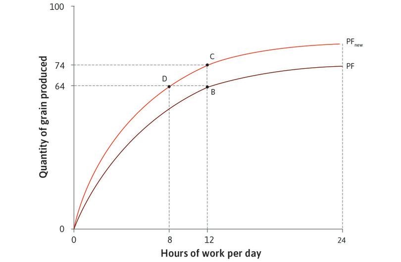
In the text, we illustrated technological progress with Figure 3.12, which we reproduce below as Figure 1. Angela’s production function shifts up, because she is able to produce more grain per hour of work.

The production function we have been working with so far (in particular in Leibniz 3.1.2) is:

$$y = Ah^\alpha$$

In this example, $h$ stands for Angela’s daily hours of work on her farm, and $y$ her daily grain output. $A$ and $\alpha$ are two parameters that describe the specific shape and position of her production function; we have assumed that $A \gt 0$ and $0 \lt \alpha \lt 1$. The first assumption simply means that work translates into creating, not destroying grain. The second assumption imposes diminishing marginal product of labour, so the production function has a concave shape.

Technological progress is being able to produce more with the same quantity of inputs: the production function will now match a higher quantity of grain to the same number of hours worked. Mathematically, there are two ways to achieve this with Angela’s production function.

If $A$ increases, then output also increase for any given level of hours worked. Thus an increase in $A$ can be interpreted as technological progress.

If $\alpha$ increases, then output decreases if $0 \lt h \lt 1$ and increases if $h \gt 1$. If we interpret the unit of measurement of $h$ literally to be an hour, then $h \gt 1$ would appear to be the normal case, so an increase in $\alpha$ may also be interpreted as technological progress.

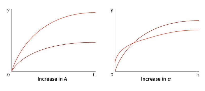
The two different ways to model technological progress are sketched in the two panels of Figure 2. In the left-hand panel, an increase in $A$ increases $y$ by the same multiple at every value of $h$. For example, if $\alpha=\frac{1}{2}$ and $A$ increases from $1$ to $2$, then $y$ changes from $\sqrt{h}$ to $2\sqrt{h}$, a 100% increase in output for any given amount of work. In the right-hand panel, an increase in $\alpha$, with $A$ held constant, increases $y$ for any $h\gt1$: if, for example, $A = 1$, $h=8$ and $\alpha$ increases from $\frac{1}{3}$ to $\frac{1}{2}$, then Angela’s daily production of grain rises from $2$ to $2\sqrt{2}$ units, a little more than 40%.

The two panels of Figure 2 show that increasing $A$ and increasing $\alpha$ have similar but not identical effects. The parameter $\alpha$ determines the curvature of the function. When $\alpha\lt1$, as we have assumed, it is concave. But if $\alpha=1$ it is a straight line, and when $\alpha\gt1$ it is convex. If $\alpha$ is initially less than 1, and then increases a little, the curve becomes less concave. The economic meaning of this is that if Angela increases her daily hours of work, diminishing marginal returns kick in less rapidly than they would have done with the smaller value of $\alpha$.

Indeed, if $\alpha$ continued to rise, becoming equal to and then greater than $1$, diminishing returns would cease to apply. This suggests that modelling technological progress as an increase in $\alpha$ is problematic for a reason rather more profound than the one stated above about what happens if $h\lt1$: human society has been experiencing technological progress for centuries now, and yet we still face diminishing returns to our labour. Assuming that technological change can free us from concavity of the production function is simply not very plausible.

Modelling technical progress as a change in $A$ avoids this problem. In this case $y$ increases at any given $h\gt0$ and the production function remains concave: the property of diminishing marginal product still holds. This is why economists normally use $A$ and not $\alpha$ to model technological change.

We can model technological change in the same way for any production function. Suppose the production function is:

$$y=Af(h)$$

where $f$ is any increasing concave function taking positive values for all $h\gt0$. Then an increase in the parameter $A$ implies that output increases by the same proportion for every level of $h$.

The property of diminishing marginal product is preserved under technological change in this general case too. The marginal product of labour (MPL) is $Af'(h)$. Thus if hours of work change from $h_0$ to $h_1$, the proportional change in the MPL is:

$$\frac{Af'(h_1) - Af'(h_0)}{Af'(h_0)} = \frac{f'(h_1) - f'(h_0)}{f'(h_0)}$$

which does not depend on $A$. Thus if $A$ increases, there is no effect on the proportional fall in the MPL caused by an increase in hours.

Read more: Sections 4.3 and 7.3 of Malcolm Pemberton and Nicholas Rau. 2015. Mathematics for economists: An introductory textbook, 4th ed. Manchester: Manchester University Press.