Leibniz

7.4.1 Isoprofit curves and their slopes

A firm’s profit is the difference between its revenue (the price multiplied by quantity sold) and its total costs. If we know the firm’s cost function, $C(Q)$, we can determine its isoprofit curves—the combinations of $P$ and $Q$ that give the same amount of profit. In this Leibniz, we obtain the equation of an isoprofit curve, explain its shape and find its slope.

Economic profit is revenue minus costs. For a manufacturing firm such as Beautiful Cars, profit depends on the quantity of output produced ($Q$) and the price ($P$) at which each unit of output can be sold. We denote profit by $\Pi,$ as before. If the firm’s cost function is $C(Q)$, then its profit can be written as a function of $P$ and $Q$:

$$\Pi = PQ - C(Q)$$

The isoprofit curves are a family of curves in the $QP$-plane, each of which corresponds to a given level of profit. The equation of a typical isoprofit curve is:

$$PQ - C(Q) = k$$

where $k$ is a constant representing the level of profit. There is a different curve for each value of $k$. We will represent the isoprofit curves in a diagram with $P$ on the vertical axis, so it is helpful to rewrite this equation in a form that expresses $P$ as a function of $Q$:

$$P = \frac{C(Q) + k}{Q}$$

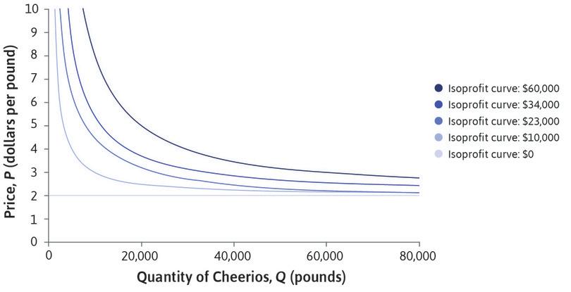
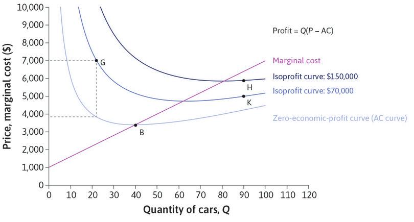
This equation implies that if $k$ increases, then $P$ also increases for any given $Q$. This means that in a diagram depicting the family of isoprofit curves, higher curves correspond to higher levels of profit. You can see this in the diagrams in the text for Apple Cinnamon Cheerios (Figure 7.4) and Beautiful Cars (Figure 7.10) of the text, reproduced here as Figures 1 and 2.

We now explain why the isoprofit curves for these two firms have the shapes shown in this diagram. The equation of the isoprofit curve corresponding to the level of profit $k$ may be written:

$$P = \frac{C(Q)}{Q} + \frac{k}{Q}$$

or equivalently

$$P = \text{AC} + \frac{k}{Q}$$

Focus first on the case where $k = 0$: the zero-economic-profit curve. Setting $k = 0$ in the equation above shows that the zero-economic-profit curve is the average cost (AC) curve. At all points below this curve in the diagram, the firm would be making a loss. For Apple Cinnamon Cheerios the average cost is constant: each pound costs $2 to produce, whether the total quantity is large or small. So the zero-economic-profit curve is a horizontal line at $P = 2$. Beautiful Cars has a U-shaped average cost curve and hence a U-shaped zero-economic-profit curve.

Now consider the curves corresponding to positive levels of profit, $k\gt0.$ Then the equation of the isoprofit curve expresses $P$ as the sum of AC and $k/Q$. Notice that $k/Q$ is high when $Q$ is small, and

$$\frac{d}{dQ} \left( \frac{k}{Q} \right) = - \frac{k}{Q^2} \lt0, \quad \frac{d^2}{dQ^2} \left( \frac{k}{Q} \right) = \frac{2k}{Q^3} \gt0$$

So $k/Q$ is a decreasing, convex function of $Q$.

The shape of the isoprofit curves depends on the shapes of $k/Q$ and the AC curve. In the case of Apple Cinnamon Cheerios this is particularly simple. AC is a horizontal line and the equation of the isoprofit curves is $P = 2+k/Q$. So the isoprofit curves are decreasing and convex, like $k/Q$, as we see in Figure 1.

For Beautiful Cars the AC curve is U-shaped, and therefore convex, with a minimum point at $Q = 40$ (point B). The isoprofit curve corresponding to a level of profit $k\gt0$ must then be convex too, since the sum of two convex functions is always convex (the second derivative of $f(x) + g(x)$ is $f''(x) + g''(x)$, which is positive if $f''(x)$ and $g''(x)$ are positive).

If $0\lt Q\lt40$, both $C(Q)/Q$ and $k/Q$ are decreasing functions of $Q$, so the isoprofit curve slopes downward. If $Q$ is large, the derivative of $k/Q$ is close to zero, so the slope of the isoprofit curve is almost the same as the slope of $C(Q)/Q$—the isoprofit curve slopes upward (as does the AC curve). Hence the isoprofit curve for $k\gt0$, like the AC curve, is U-shaped, with a minimum point at some positive value of $Q$.

Let $Q^*$ be the value of $Q$ where the minimum occurs. Notice that $Q^*$ depends on $k$. We know that all the isoprofit curves slope downward until $Q = 40$, so $Q^* \gt 40$: the minimum point on an isoprofit curve with $k\gt0$ is to the right of the minimum point of the zero-profit curve. A similar argument shows that as we increase $k$, $Q^*$ also increases: isoprofit curves corresponding to higher levels of profit have their minimum point further to the right (Figure 2).

We have now explained why the isoprofit curves for Beautiful Cars are U-shaped. The other property you can see in Figure 2 is that the marginal cost curve passes through the minimum points of the isoprofit curves. In Leibniz 7.3.1 we proved that this is true for the AC curve (the zero-isoprofit-curve) by showing that $\text{MC} - \text{AC}$ always has the same sign as the slope of the AC curve. We now use the same approach for the slopes of the other isoprofit curves.

Consider the isoprofit curve corresponding to a profit of $k\gt0$. Along this curve:

$$\frac{dP}{dQ} = \frac{d} {dQ} \left( \frac{C(Q)}{Q} \right) - \frac{k}{Q^2}$$

Thus $dP/dQ$ is the difference of two terms, the first of which is the slope of the AC curve; we showed in Leibniz 7.3.1 (using the quotient rule) that this is $(\text{MC} - \text{AC)}/Q$. Also, we know from the equation of the isoprofit curve that $k/Q = P - \text{AC}$. Therefore:

$$\frac{dP}{dQ} = \frac{\text{MC} - \text{AC}}{Q} - \frac{P - \text{AC}}{Q}$$

Simplifying the right-hand side, we see that:

$$\frac{dP}{dQ} = \frac{\text{MC} - P}{Q}$$

This equation tells us the slope at any point on the isoprofit curve $P = \text{AC}+ k/Q$. When $Q$ is small $P$ is high—above marginal cost MC—and the curve slopes down. So as $Q$ increases, $P$ decreases; this continues as long as $P\lt \text{MC}$. In the case of Beautiful Cars we eventually reach a point where $P = \text{MC}$ and at that point, the equation tells us that the slope is zero: we have reached a minimum point of the isoprofit curve. The MC-curve slopes upward through this point. And so beyond this point, $\text{MC} \gt P$ and the isoprofit curve slopes upward too.

What about the case of Apple Cinnamon Cheerios? Since the unit cost of a pound of Cheerios is $2 whatever the level of production, both the marginal and average cost is $2. The zero-isoprofit-curve is not only the AC-curve, but the MC-curve as well. The equation of any isoprofit curve can be written as $P = \text{MC}+ k/Q$. So if $k \gt 0$, then $P \gt \text{MC}$, which means that the slope is always negative. As you can see in Figure 1, all the positive isoprofit curves slope downward, but never meet the MC-curve.

Read more: Chapter 8 of Malcolm Pemberton and Nicholas Rau. 2015. Mathematics for economists: An introductory textbook, 4th ed. Manchester: Manchester University Press.